η Broadening Artifact

The TBtrans Green function is computed as

$$G^r(E) = \left[(E + i\eta)\,S - H - \Sigma_L - \Sigma_R\right]^{-1}$$

where $\eta$ (TBT.Contours.Eta) is a numerical imaginary part that stabilizes the matrix inversion. It is not a physical quantity. Since $\eta$ broadens spectral structure with a Lorentzian width $\sim\eta$, an excessive $\eta$ can qualitatively distort the interpretation in systems with sharp resonances, band edges, or 1D van Hove singularities whose physical widths are narrower than $\eta$.

Symptoms of excessive η

Symptom	Mechanism
Sharp resonances and band edges are excessively broadened	Lorentzian convolution — structures narrower than $\eta$ cannot be resolved
Artificial suppression of $T(E)$	Near band edges, spectral weight leaks into the gap, making channels appear less open
Loss of ballistic plateaus	Even in a perfectly periodic system, integer $T$ is shaved below the integers and corners are rounded
Artificial length dependence	Broadened resonance tails decay differently with device length — as the length grows, it looks like an exponential decay in which $T$ keeps shrinking

The last symptom is especially dangerous. The observation "$T(E_F)$ decreases exponentially with device length" reads plausibly as tunneling physics, but if such a trend appears in a pristine system that should be ballistic, suspect an $\eta$ artifact rather than physics. In that state, the scattering region length convergence judgment itself is impossible.

Diagnostic procedure

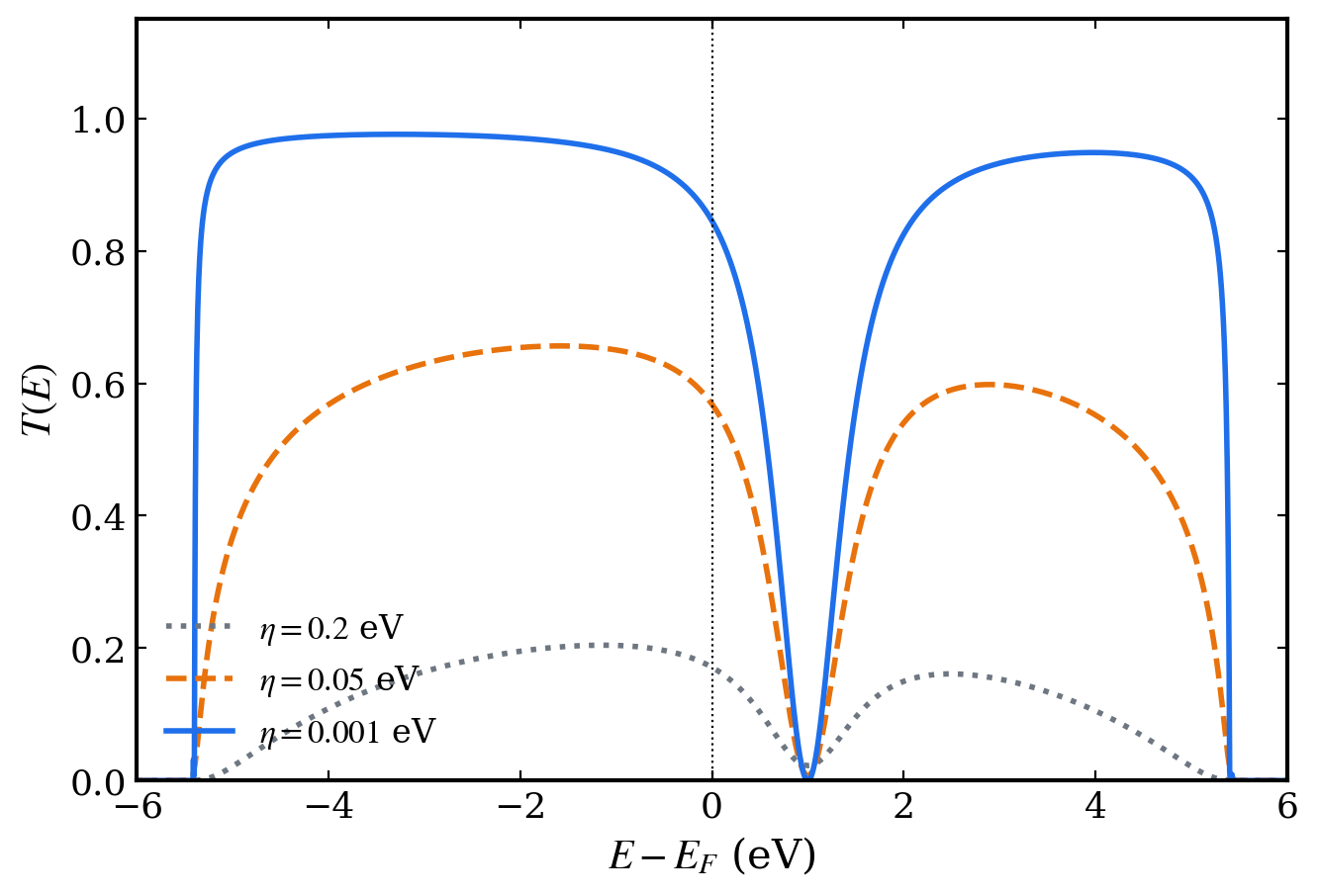
Figure 1. $T(E)$ of the same device with a coupled local level, computed at $\eta$ = 0.2 / 0.05 / 0.001 eV — an excessive $\eta$ artificially lowers the plateau and distorts the dip structure by broadening it. Check whether the curves converge as $\eta$ is lowered. (Actual TB-model calculation, _scripts/fig_examples_batch.py)

1. η series — compute the same system while lowering $\eta = 0.05 \rightarrow 0.005 \rightarrow 0.001$ eV and overlay the $T(E)$ curves. Convergence is the point where the curve no longer depends on $\eta$. If lowering $\eta$ by one step changes the result substantially, the previous value was excessive.
2. Ballistic litmus — confirm that $T(E)$ recovers integer plateaus in the pristine chain without impurities. The $T(E)$ of a perfect 1D crystal must equal the number of bands at that energy. If the plateau is shaved down, $\eta$ is still too large.
3. Shrink the energy grid along with it — lowering $\eta$ narrows the spectral structures, so the energy grid spacing delta must be reduced together. Peaks narrower than the grid are missed by the sampling or alias into jagged spikes. Rule of thumb: keep delta at or below the same order of magnitude as $\eta$. The standard setting of this tutorial ($\eta = 0.001$ eV, delta $= 0.001$ eV) is an example.
4. Re-examine the length dependence — after $\eta$ convergence, rerun the length series and confirm that the previously observed length dependence disappears.

Easily confused points

• The contour method is unrelated to $T(E)$. The energy-integration quadrature scheme (simpson, mid-rule, etc.) has no effect on the values of the $T(E)$ curve; it affects only the accuracy of the current integral $I = \int T(E)\,[f_L - f_R]\,dE$. Changing the quadrature when the shape of $T(E)$ looks wrong is a prescription unrelated to the cause.
• The η of the electrode self-energy is separate. The recursive computation of the electrode surface Green function has its own broadening, set independently of the device's $\eta$. Check the default coupling rule and the option names in the TBtrans manual.
• η cannot be negative. By the definition of the retarded Green function, only positive values are valid.

The special nature of 1D systems

In 3D/2D junctions, the transverse k-point average naturally smooths the spectrum, so the relative influence of $\eta$ is small. In contrast, a 1D chain isolated by vacuum has no transverse k average and is particularly sensitive to $\eta$ convergence. The $1/\sqrt{E}$ van Hove singularities at 1D band edges also create narrow structures. This tutorial therefore starts at $\eta = 0.001$ eV, but demands a per-system convergence check without exception. A smaller $\eta$ requires a denser energy grid, and the computational cost can be managed with TBtrans energy-point parallelization.

References

• TBtrans User Guide: https://docs.siesta-project.org/ — TBT.Contours.Eta and the electrode broadening options
• S. Datta, Electronic Transport in Mesoscopic Systems (Cambridge University Press, 1995) — general theory of broadening and level width