Mini-project: polyyne–cumulene junction

This is the capstone project that runs through the entire tutorial. Build a junction with a semiconducting polyyne segment sandwiched between metallic cumulene electrodes, run the full workflow yourself from the electrode calculation to eigenchannel analysis, and extract the tunneling decay constant $\beta$. The operating instructions for each step are already in the corresponding chapters, so this document focuses on the project's flow, analysis, and checkpoints.

Project objectives

• Reuse the cumulene electrode (Chapter 05) and complete the full chain — 0 V TranSIESTA → TBtrans → I–V → eigenchannel — for a 6-atom polyyne junction.
• Confirm from $T(E)$ and the eigenchannels that the polyyne segment acts as a tunneling barrier.
• Confirm the exponential decay of $T(E_F)$ in a polyyne length series of 4/6/8 atoms and extract the decay constant $\beta$.

Physical background — Peierls relaxation and the tunneling barrier

An infinite carbon atomic chain can take two bonding patterns.

• cumulene — all bonds equally spaced ($d = 1.29\ \text{Å}$). It is a metal with two degenerate $\pi$ bands passing through $E_F$. This is precisely the electrode structure of the main tutorial.
• polyyne — a structure with alternating bond lengths (bond-length alternation, BLA). Here we use $1.24/1.34\ \text{Å}$.

A one-dimensional metal is unstable against lattice dimerization — the Peierls instability. When an equally spaced chain dimerizes, the $\pi$ bands split at the Brillouin zone boundary, a gap opens at $E_F$, and the system lowers its total energy. The size of the gap is sensitive to the BLA.

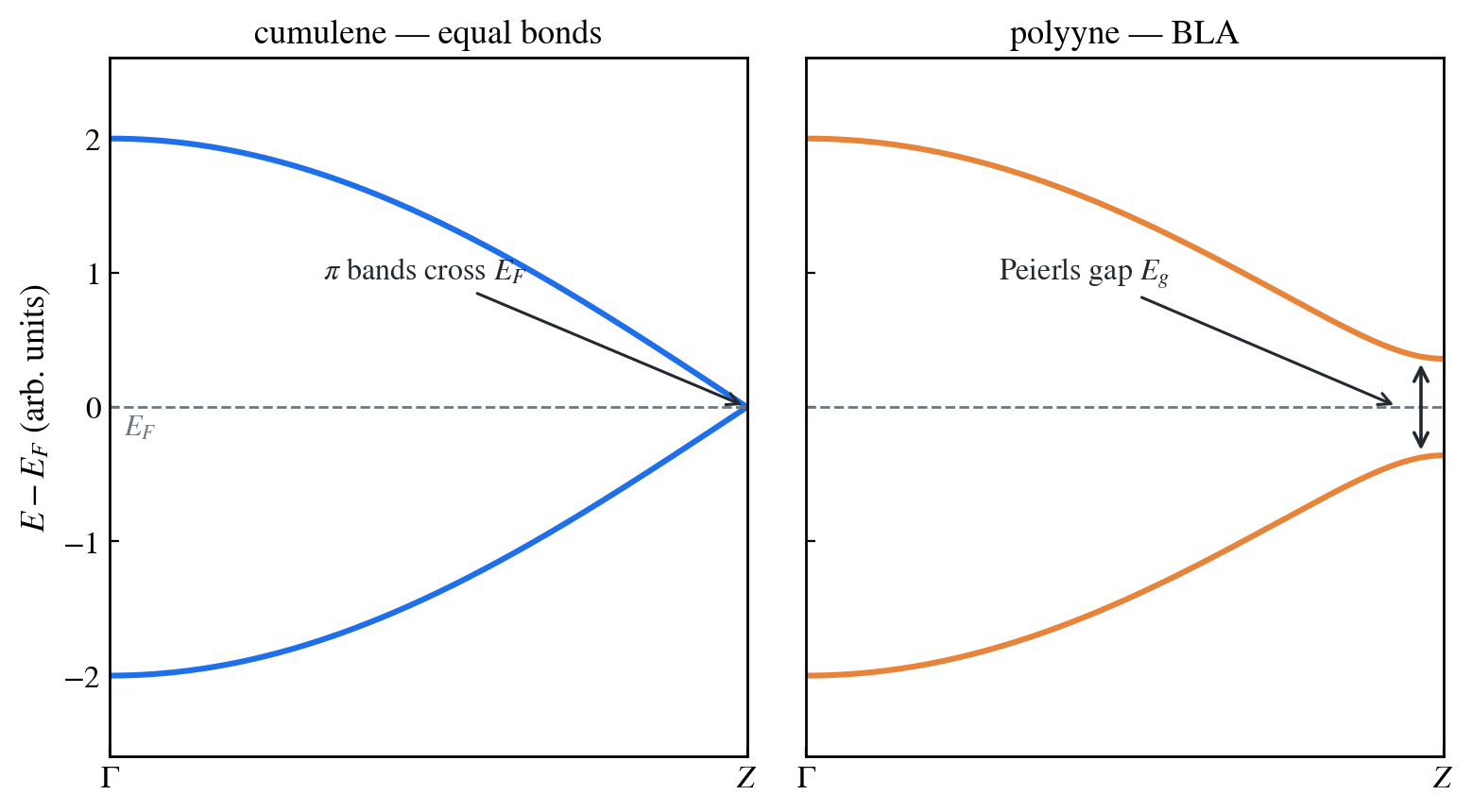
Figure 1. Band shapes of cumulene (metal) and polyyne (BLA, gap) (tight-binding conceptual diagram) — the design rationale of this junction is that the electrode is a metal crossing $E_F$ while the scattering region is a barrier with an open gap.

The junction of this project turns that contrast directly into a device. Placing a segment with an open gap (polyyne) between metals (cumulene electrodes) means that electrons near $E_F$ cannot exist as propagating waves in the polyyne section and pass through as evanescent states while decaying. The result is the universal form of tunneling.

$$T(E_F) \approx T_c\, e^{-\beta L}$$

$L$ is the barrier (polyyne section) length and $T_c$ is the prefactor set by the contacts. $\beta$ is determined by the decay rate $\kappa$ of the evanescent states inside the barrier ($\beta = 2\kappa(E_F)$), an intrinsic quantity set by the complex band structure of the barrier material (Tomfohr & Sankey, Phys. Rev. B 65, 245105 (2002)). The larger the gap and the closer $E_F$ is to the middle of the gap, the larger $\beta$. The final deliverable of this project is the $\beta$ measured from the length series.

System definition

The device is the C19N structure of the main tutorial (Chapter 06) with only the scattering region replaced by polyyne. The electrodes and the computational standards (DZP, MeshCutoff 300 Ry, SCF.DM.Tolerance 1.0d-8, PseudoDojo PBE C.psml) are the same as in the main tutorial.

Region	Composition	Remarks
Left electrode	cumulene C, 8 atoms (2 cells, $d = 1.29\ \text{Å}$)	The Chapter 05 electrode verbatim
Scattering region	polyyne C, $N$ atoms, bonds alternating $1.24/1.34\ \text{Å}$	Arranged so that the bonds at both ends are triple ($1.24\ \text{Å}$)
Right electrode	cumulene C, 8 atoms (2 cells)	Identical to the left
Interface bond	Fixed at $1.29\ \text{Å}$	The cumulene value. Unrelaxed ideal geometry (see the note below)

If the number of polyyne atoms is even, the number of internal bonds is odd, so the bond sequence is a palindrome and the whole junction becomes a left–right mirror-symmetric symmetric junction. The length series is as follows.

case	Number of atoms	Polyyne section length $L$ ($\text{Å}$)	cell $c$ ($\text{Å}$)
p4	20	3.82	25.75
p6	22	6.40	28.33
p8	24	8.98	30.91

$L$ is defined as the distance between the first and last polyyne atoms. The structure-generation script (build_polyyne_junction.py) and the three struct files are in the repository's code/miniproject/. The p6 structure is as follows.

struct_p6.fdf

# polyyne(6C)-cumulene junction device -- generated by build_polyyne_junction.py
# left cumulene 8C + polyyne 6C (1.24/1.34 Ang) + right cumulene 8C, interface 1.29 Ang
# ideal (unrelaxed) geometry, chain at (7.5, 7.5) Ang, transport along z
NumberOfAtoms    22
NumberOfSpecies  1

%block ChemicalSpeciesLabel
  1  6  C
%endblock ChemicalSpeciesLabel

LatticeConstant 1.0 Ang
%block LatticeVectors
  15.000000   0.000000    0.000000
   0.000000  15.000000    0.000000
   0.000000   0.000000   28.330000
%endblock LatticeVectors

AtomicCoordinatesFormat Ang
%block AtomicCoordinatesAndAtomicSpecies
   7.500000   7.500000   0.000000  1
   7.500000   7.500000   1.290000  1
   7.500000   7.500000   2.580000  1
   7.500000   7.500000   3.870000  1
   7.500000   7.500000   5.160000  1
   7.500000   7.500000   6.450000  1
   7.500000   7.500000   7.740000  1
   7.500000   7.500000   9.030000  1
   7.500000   7.500000  10.320000  1
   7.500000   7.500000  11.560000  1
   7.500000   7.500000  12.900000  1
   7.500000   7.500000  14.140000  1
   7.500000   7.500000  15.480000  1
   7.500000   7.500000  16.720000  1
   7.500000   7.500000  18.010000  1
   7.500000   7.500000  19.300000  1
   7.500000   7.500000  20.590000  1
   7.500000   7.500000  21.880000  1
   7.500000   7.500000  23.170000  1
   7.500000   7.500000  24.460000  1
   7.500000   7.500000  25.750000  1
   7.500000   7.500000  27.040000  1
%endblock AtomicCoordinatesAndAtomicSpecies

Atoms 1–8 are the left electrode, 9–14 the polyyne (the section where the spacing alternates as $1.24/1.34$), and 15–22 the right electrode. Use these numbers when filling in atom-range blocks such as %block TBT.Atoms.Device.

Figure 2. The ideal geometry of the p6 junction (struct_p6.fdf rendering, 22 C atoms) — between the 8-atom cumulene electrodes on both sides ($d = 1.29$ Å), the bond lengths of the central 6-atom polyyne section (atoms 9–14) alternate as $1.24/1.34$ Å (BLA).

On the interface geometry

Fixing the interface bond at $1.29\ \text{Å}$ is a pedagogical choice that keeps the definition of $\beta$ clean. In actual research you would relax the whole junction (Chapter 03) and reflect how the BLA relaxes at the interface, which changes $T_c$ (the prefactor). This is treated in extension task 1.

The recommended directory structure follows the convention of the main tutorial.

miniproject/
├── 01_electrode/          # cumulene electrode of Chapter 05 (reused)
├── p4/
│   └── 0bias/             # TranSIESTA 0 V + TBtrans
├── p6/
│   └── 0bias/
└── p8/
    └── 0bias/

Step-by-step procedure

Step 1 — Electrode (reuse)

Use the cumulene electrode of Chapter 05 (4 C atoms, $c = 5.16\ \text{Å}$, SystemLabel Electrode) verbatim. If you already computed it in the main tutorial, there is no need to recompute Electrode.TSHS — every case references the same electrode file by relative path.

Checkpoint: Electrode.TSHS exists. Confirm with the approach of Chapter 02 that the electrode bands are metallic, crossing $E_F$ (two cumulene $\pi$ bands).

Step 2 — Device 0 V TranSIESTA

In the 0bias/ setup of Chapter 06, change only the structure file to struct_p6.fdf. Since the atom count grows from 20 to 22, the blocks containing atom ranges (electrode region specification, TBT.Atoms.Device, etc.) must be updated to the 22-atom basis — omitting this range update is the most common mistake.

Checkpoint: SCF convergence (by the SCF.DM.Tolerance 1.0d-8 criterion), trans.TSHS generated. Whether the potential and density of the electrode regions inside the device (atoms 1–8, 15–22) match the bulk electrode — if the scattering region encroaches on the electrodes, extend the electrode cell as in Advanced: scattering region convergence.

Step 3 — TBtrans $T(E)$

Run exactly as in Chapter 07. Tutorial standard: energy grid $[-3, 3]\ \mathrm{eV}$, TBT.Contours.Eta 0.001 eV, grid spacing finer than $\eta$.

Checkpoint: Whether $T(E)$ is strongly suppressed in the gap energy region around $E_F$ ($T(E_F) \ll 1$) and recovers outside the gap, i.e., a barrier shape. Overlaying it with the $T(E)$ of C19N from the main tutorial makes the difference between "impurity scattering" and "gap tunneling" visible at a glance.

Step 4 — I–V (symmetric window)

Apply iv_zerobias.py of Chapter 08 verbatim. Keep the symmetric window convention $\mu_{L,R} = E_F \pm eV/2$.

Checkpoint: Antisymmetry $I(-V) = -I(V)$ holds — this junction is mirror-symmetric, so any asymmetry means the window convention is wrong. The low-bias slope agrees with $G_0\,T(E_F)$. At the same bias, the current is orders of magnitude smaller than for C19N of the main tutorial (because it is a barrier).

Step 5 — Eigenchannel

Decompose and visualize the eigenchannels at $E_F$ following the approach of Chapter 10.

Checkpoint: The transmission eigenvalues $\tau_n$ of the top two channels (the degenerate $\pi_x/\pi_y$) are close to each other and both far below 1. The $z$-profile of $|\psi|^2$ is large in the left electrode and decays exponentially as it passes through the polyyne section — the real-space picture of tunneling.

Step 6 — Length series and extraction of $\beta$

Repeat steps 2–3 with struct_p4.fdf and struct_p8.fdf (note that the atom count, range blocks, and cell length differ for each case). Collect $T(E_F)$ of the three cases and fit a straight line to $\ln T(E_F)$ versus $L$.

beta_fit.py

"""Extract the tunneling decay constant beta from the polyyne length series."""
import numpy as np
import sisl

cases = {4: 3.82, 6: 6.40, 8: 8.98}   # N -> polyyne section length L (Ang)

L, lnT = [], []
for N, length in sorted(cases.items()):
    tbt = sisl.get_sile(f"p{N}/0bias/trans.TBT.nc")
    E = np.asarray(tbt.E)                    # E - E_F (eV)
    T = np.asarray(tbt.transmission())
    TEf = np.interp(0.0, E, T)               # T(E_F)
    L.append(length)
    lnT.append(np.log(TEf))
    print(f"p{N}: T(E_F) = {TEf:.3e}")

slope, intercept = np.polyfit(L, lnT, 1)
print(f"beta = {-slope:.3f} 1/Ang   (T_c = {np.exp(intercept):.3f})")

Checkpoint: The three points lie on a straight line in the $\ln T$–$L$ plane (the criterion for exponential decay). A large fit residual means you are still in the short-length regime where contact effects dominate.

The form of the expected results

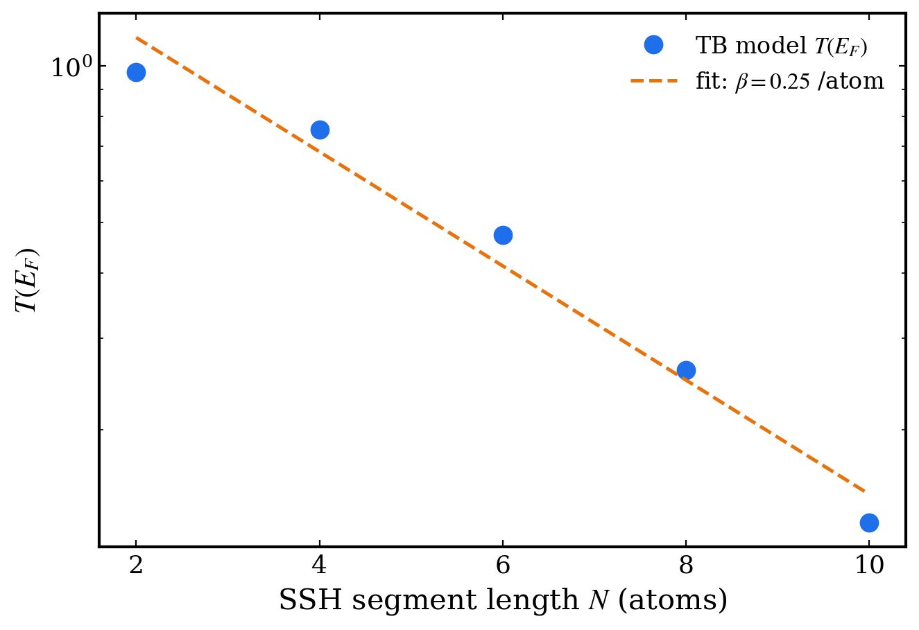
Figure 3. $T(E_F)$ versus SSH (polyyne-type) segment length — a straight line on a semilog scale means exponential decay, and the slope is the decay constant $\beta \approx 0.25$/atom (a TB-model value — different from the $\beta$ of a DFT result). This is the form of the result you will obtain in this mini-project. (_scripts/fig_examples_batch.py)

Since the specific numbers depend on basis, functional, and geometry, what judges the results is the following forms.

• $T(E)$: a deep valley in the energy region containing $E_F$ (the polyyne gap), with $T$ recovering above 1 outside the gap edges. The longer the polyyne, the lower $T$ inside the gap, while the position and width of the gap stay nearly the same — this must agree with the tunneling picture in which lengthening the barrier does not change the barrier height.
• I–V: a low current, antisymmetric about the origin. Linear at low bias, growing superlinearly as the window approaches the gap edges.
• Eigenchannel: a $|\psi|^2$ that decays monotonically and exponentially in the polyyne section.
• $\beta$: a consistent positive value across the three lengths. Since it is tunneling through the gap created by the BLA, increasing the gap (extension task 3) must also increase $\beta$.

Checkpoint summary

Step	Deliverable	Pass criterion
1. Electrode	Electrode.TSHS	Bands cross $E_F$ (metallic)
2. Device 0 V	trans.TSHS	SCF converged, electrode regions inside the device are bulk-like
3. TBtrans	trans.TBT.nc	A gap valley in $T(E)$, $T(E_F) \ll 1$
4. I–V	iv_zerobias.dat	$I(-V) = -I(V)$, low-bias slope $= G_0 T(E_F)$
5. Eigenchannel	Per-channel $\tau_n$, $\lvert\psi\rvert^2$ profile	Exponential decay in the polyyne section
6. Series	$\beta$	Linearity of $\ln T(E_F)$ versus $L$

Extension tasks

1. Interface relaxation. Relax the p6 junction following the approach of Chapter 03, then repeat steps 2–3. How do the interface bond and the nearby BLA change, and what effect does that have on $T(E_F)$ and on the prefactor $T_c$ of the $\beta$ fit?

2. Finite bias. Apply the bias chain of Chapter 09 to p6 and compare with the zero-bias-approximation I–V. At what bias do the two results begin to diverge in a barrier junction?

3. BLA and $\beta$. Rebuild the series with a reduced-BLA structure ($1.27/1.31\ \text{Å}$) and extract $\beta$ (you only need to change D_TRIPLE/D_SINGLE in build_polyyne_junction.py). Check whether the trend of $\beta$ decreasing as the gap shrinks agrees with the complex band picture.

---

Ref: R. E. Peierls, Quantum Theory of Solids (Oxford UP, 1955) (Peierls instability); J. K. Tomfohr and O. F. Sankey, Phys. Rev. B 65, 245105 (2002) (complex bands and the decay constant); S. Datta, Quantum Transport: Atom to Transistor (Cambridge UP, 2005).