IP/EA Calculations — the Raw Material of ΔSCF and Level Alignment

In the DFT+Σ correction of Chapter 11, the magnitude of the gas-phase component $\Sigma^1$ comes from the difference between the IP (ionization potential)/EA (electron affinity) of the isolated molecule and the DFT eigenvalue. How that IP/EA is actually computed is the subject of this chapter. The method itself is the simple definition of a total-energy difference (ΔSCF), but the practice of handling charged cells in a periodic-boundary code (VASP) has several known pitfalls. The order here is: definition → difference from the Koopmans approximation → the VASP ΔSCF procedure → the limits of charged-cell corrections → image-charge renormalization inside a junction.

Learning objectives

• Define IP/EA as total-energy differences and explain the difference from the Koopmans approximation ($-\varepsilon_{\mathrm{HOMO}}$).
• Carry out the procedure of computing ΔSCF IP/EA in VASP by changing the electron count with NELECT.
• Know the artificial electrostatic interaction of charged cells under periodic boundaries and the limits of its correction (box-size extrapolation).
• Explain the direction and order of magnitude of the renormalization of gas-phase IP/EA by electrode screening inside a junction.

Definition — the total-energy difference is the definition

The IP and EA of an $N$-electron system are defined as ground-state total-energy differences between systems with different electron counts.

$$\mathrm{IP} = E(N-1) - E(N), \qquad \mathrm{EA} = E(N) - E(N+1)$$

Because they are obtained by subtracting the total energies of two (or three) SCF calculations, this is called ΔSCF. There are two kinds, depending on when the structure is held fixed.

• vertical — the neutral equilibrium structure is held fixed and only the electron count is changed. This corresponds to the vertical transition of photoelectron spectroscopy, and it is the value that enters the level-alignment correction of Chapter 11 (the structure of a molecule inside a junction has no time to relax at the instant of charging).
• adiabatic — the structure is relaxed again in the charged state. This corresponds to the thermodynamic ionization energy.

For the purpose of this chapter (raw material for level correction) we use vertical. Always state which one was used when reporting results.

The difference between the two values is the fundamental gap of the molecule.

$$E_{\mathrm{gap}}^{\mathrm{fund}} = \mathrm{IP} - \mathrm{EA}$$

What was called the "gas-phase gap" in Chapter 11 is exactly this quantity, and that the PBE Kohn–Sham gap is much smaller than it was the first motivation for DFT+Σ.

The Koopmans approximation and its failure

As a shortcut for reading the IP off a single DFT calculation, $-\varepsilon_{\mathrm{HOMO}}$ (the Koopmans approximation) is often used. In exact Kohn–Sham theory, $-\varepsilon_{\mathrm{HOMO}} = \mathrm{IP}$ holds as a theorem, but the self-interaction error of semi-local functionals pushes occupied levels upward and badly breaks this relation. Benzene is the well-known example.

Method	Benzene IP estimate (eV, approximate)	Remarks
Experiment (vertical)	9.2	Photoelectron spectroscopy
ΔSCF (PBE)	around 9.2	Total-energy difference — close to experiment thanks to error cancellation
$-\varepsilon_{\mathrm{HOMO}}$ (PBE)	low 6s	Underestimated by about 3 eV — self-interaction error
$-\varepsilon_{\mathrm{HOMO}}$ (hybrid, B3LYP/PBE0)	7s	Improves in proportion to the exact-exchange mixing, but still underestimates

Two points. First, PBE's $-\varepsilon_{\mathrm{HOMO}}$ underestimates the IP by several eV, so it cannot be used as-is as the reference for level correction. Second, even with the same PBE, ΔSCF is a total-energy difference, so the errors largely cancel and it comes much closer to experiment for small molecules — the reason the gas-phase component of DFT+Σ is based on ΔSCF (or an approximation mediated by hybrid eigenvalues, Chapter 11) rather than on eigenvalues.

It is worth noting why ΔSCF works. The total energy of a semi-local functional is relatively accurate at integer electron counts, and the two errors carried by the eigenvalues — self-interaction and the missing derivative discontinuity (Chapter 11) — largely cancel in the difference between $E(N-1)$ and $E(N)$. That is, ΔSCF is a strategy that bypasses the eigenvalues and uses only the more trustworthy side of the functional, the total energy. This cancellation is an empirical tendency rather than a guarantee, however, so present a comparison against the experimental vertical IP wherever the system allows it.

Practical procedure — VASP ΔSCF

Since an isolated molecule is treated in a periodic code, settings that suppress interactions between periodic images come first.

• Large box + $\Gamma$ point — secure at least 12 Å of vacuum measured from the molecular edge and use only the single $\Gamma$ k-point (an isolated molecule should have no dispersion).
• Electron-count control — change the electron count by $\pm1$ with NELECT. Check the default electron count of the neutral calculation from the NELECT value in OUTCAR, and add or subtract 1 from it.
• Spin polarization is mandatory — removing or adding one electron from a closed-shell molecule makes it an odd-electron system, so run the charged calculations with ISPIN = 2 and check that the final magnetic moment is the expected value (1 μB).
• smearing — molecular levels are discrete, so use ISMEAR = 0 with a small SIGMA (on the order of 0.01 eV).
• All settings identical except NELECT — the three calculations must have exactly the same ENCUT, box, SIGMA, and pseudopotential. If even one differs, that difference does not cancel and remains directly in the IP/EA (exercise 4).

INCAR (cation, N-1 electrons — for the vertical IP)

SYSTEM = molecule cation, fixed neutral geometry
PREC   = Accurate
ENCUT  = 500
ISMEAR = 0
SIGMA  = 0.01
EDIFF  = 1E-8
ISPIN  = 2
NELECT = 41        # example for a neutral system with 42 electrons -- one less than the NELECT in the neutral OUTCAR

The procedure is three single-point calculations (the structure fixed at the neutral relaxation result).

Step	Calculation	Electron count	Output
1	Neutral	$N$ (default)	$E(N)$
2	Cation	NELECT $= N-1$	$E(N-1)$ → $\mathrm{IP} = E(N-1) - E(N)$
3	Anion	NELECT $= N+1$	$E(N+1)$ → $\mathrm{EA} = E(N) - E(N+1)$

Copy the same file (the CONTCAR of the neutral relaxation) verbatim as the POSCAR of all three calculations — this is the condition the vertical definition demands. Check the electron count and the energy directly in the output.

grep NELECT OUTCAR             # the electron count this calculation actually used -- compare with the intended value
grep "E0=" OSZICAR | tail -1   # smearing-extrapolated total energy E0
grep "mag=" OSZICAR | tail -1  # final magnetic moment -- is it near 1 uB in the charged calculation?

Energy comparisons use E0 (the smearing-extrapolated value) for the same reason as in Chapter 03. If a charged calculation converged with a magnetic moment of 0, the odd-electron system has settled into a wrong spin state, so impose an initial moment and search again for the doublet solution.

Note — comparing $-\varepsilon_{\mathrm{HOMO}}$ requires prior vacuum-level alignment

ΔSCF is a total-energy difference within the same box, so the reference problem cancels automatically; but comparing the eigenvalue $\varepsilon_{\mathrm{HOMO}}$ itself with the IP requires reference alignment. Eigenvalues of a periodic code are referenced to the cell-average potential, so you must take the average value in the vacuum region of the LOCPOT saved with LVTOT as the vacuum level and read $\varepsilon_{\mathrm{HOMO}} - V_{\mathrm{vac}}$ to obtain a number comparable with the experimental IP and with other codes. The $-\varepsilon_{\mathrm{HOMO}}$ values in the table above are all based on values that went through this alignment.

Pitfalls of charged cells — using them honestly

Under periodic boundaries, a charged cell is not well defined in itself. The code automatically lays down a uniform background charge (jellium) to neutralize it, and as a result the total energy mixes in an artificial electrostatic interaction among the charged molecule, its periodic images, and the background charge. The leading term decays as $q^2/L$ with the box size $L$ (Makov–Payne).

• A box-size series is the basic prescription. Increase one box edge stepwise (e.g., 12 → 16 → 20 Å) and extrapolate $E$ against $1/L$. The neutral calculation is nearly box-independent, but the charged calculations are not, so the box convergence of IP/EA must be presented numerically.
• Use automatic correction tags only after checking. VASP has correction features for charged and dipolar cells, but the conditions of applicability differ by calculation type, so check the correction you used and its premises in the manual and state them. Either way, directly confirming convergence with a box series is the least disputable procedure.
• Anions are harder. For a molecule with a negative gas-phase EA (benzene is one), the extra electron is not bound to the molecule. In a periodic cell that electron falls into an artificial state in the vacuum region, so the result drifts as the box grows; the ΔSCF for EA is therefore trustworthy only in systems where a bound anion is confirmed. Report this limitation honestly.

Do not trust the absolute value of a charged-cell total energy

The absolute total energy of a charged-cell calculation depends on the background charge and the average-potential convention. Only the energy differences that have gone through correction and extrapolation are meaningful, and an IP/EA number that does not state the box size and the correction method cannot be reproduced.

The whole procedure summarized in one table.

Item	Setting/judgment	Rationale
Box	Vacuum of at least 12 Å + size-series extrapolation	Periodic-image and background-charge interaction $\sim q^2/L$
k-points	Single $\Gamma$ point	Isolated molecule — there should be no dispersion
Structure	All three calculations fixed at the neutral relaxed structure	The vertical definition
Spin	ISPIN = 2 for charged calculations, check the final moment	Odd-electron system
smearing	ISMEAR = 0, SIGMA on the order of 0.01 eV, compare with E0	Prevent contamination of discrete levels
EA	Trust only after a bound anion is confirmed	Influx of unbound electrons into box states

Inside a junction, the gas-phase value is not used as-is

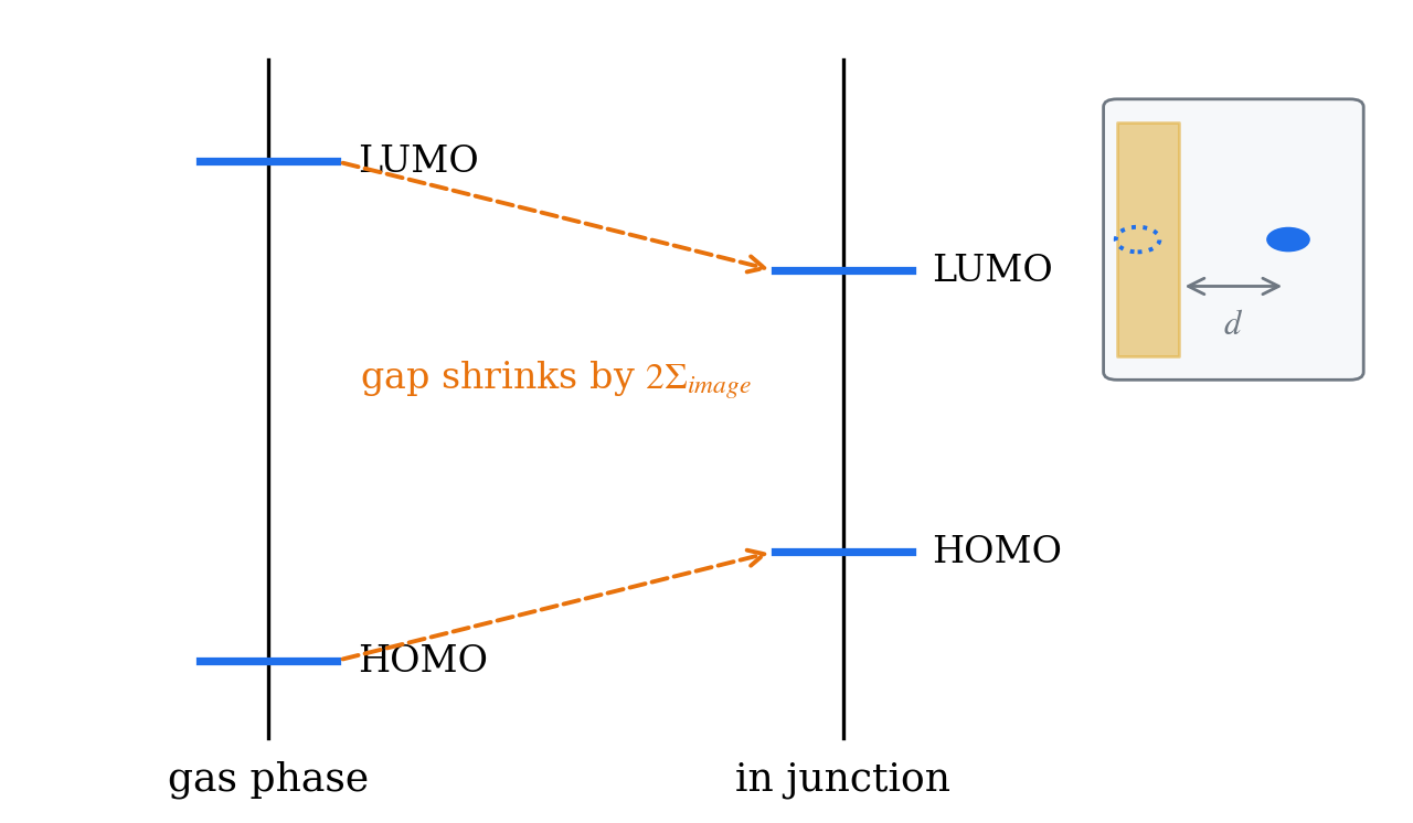
Figure 1. The picture of gas-phase HOMO/LUMO being renormalized by electrode screening inside a junction — occupied levels move up and unoccupied levels move down, narrowing the gap by $2\Sigma_{image}$. (Conceptual diagram)

The IP/EA obtained this way are values for the isolated molecule in vacuum. When the molecule is placed between metal electrodes, the image charge induced in the electrodes upon removing or adding an electron stabilizes the charged state, so occupied levels move up and unoccupied levels move down — the levels shift toward the center of the gap — and the gap becomes narrower than in the gas phase. A representative number is the GW calculation in which the gap of benzene on graphite shrinks from 10.5 eV to 7.2 eV (Neaton, Hybertsen, Louie 2006). The point of that paper is that this is a nonlocal polarization effect in which the shapes of the molecular orbitals themselves barely change while only the level positions shift by several eV — that is, an effect a semi-local functional cannot capture in principle.

Classical electrostatics suffices for the order-of-magnitude estimate. The image-charge stabilization energy of a point charge at distance $d$ from a planar metal electrode is

$$\Sigma = \frac{e^2}{16\pi\epsilon_0 d}$$

and using $e^2/4\pi\epsilon_0 = 14.4\ \mathrm{eV\cdot\text{Å}}$ gives $\Sigma \approx 3.6/d$ eV ($d$ in Å). For $d = 3$ Å this is about 1.2 eV per level — and with two electrodes the image series adds up, so the effect is larger still. Points to note:

• This formula presumes a planar metal surface with a well-defined image plane. An uncertainty of a few hundred mÅ in the image plane position swings the correction by several hundred meV, and for non-planar electrode geometries (a 1D chain electrode is the extreme example) the formula does not hold at all — exactly as seen in the limitations section of Chapter 11.
• Connecting to the notation of Chapter 11: the occupied-level correction is $W_{\mathrm{occ}} = +\Sigma$ (upward) and the unoccupied-level correction is $W_{\mathrm{virt}} = -\Sigma$ (downward). The gas-phase component $\Sigma^1$ widens the gap and the image-charge component $\Sigma^2$ narrows it again — the two components have opposite signs.
• The overall structure of the level correction is therefore a two-stage construction: (i) the gas-phase ΔSCF of this chapter provides $\Sigma^1$, and (ii) an image-charge model matched to the electrode geometry provides $\Sigma^2$. Reporting separately which approximation (box size and correction, image plane position) was used for which component is what makes the result verifiable.

Position in the pipeline

Let us restate where the deliverable of this chapter goes. In the correction formula of Chapter 11, the gas-phase ΔSCF IP/EA determines the term $\Sigma^1 = (-\mathrm{IP} - \varepsilon_{\mathrm{HOMO}}^{\mathrm{DFT}})$ (the unoccupied side corresponds via the EA), and the image-charge estimate of this chapter's last section determines $\Sigma^2$. That is, the error bar of the IP/EA calculation becomes directly the error bar of the corrected resonance position, and $T(E_F)$ inside the gap is sensitive to that position at the order-of-magnitude level — the reason box convergence and an explicit statement of the correction method are not a formality but the confidence interval of the result itself.

Exercises

1. Compute the vertical IP by ΔSCF for one small closed-shell molecule (e.g., benzene) and compare it with $-\varepsilon_{\mathrm{HOMO}}$ (PBE) from the same calculation. Check whether the difference between the two values matches the trend in the table in the text.
2. Repeat the cation calculation with box edges of 12, 16, and 20 Å, plot $E(N-1)$ against $1/L$, and report the difference between the extrapolated value and the 12 Å value (= the box finite-size error) in eV.
3. Assuming electrode–molecule distances $d$ of 2.5, 3.0, and 4.0 Å, compute $\Sigma^2$ per level with the planar image-charge formula. Organize, with signs, the fact that the gas-phase correction $\Sigma^1$ widens the gap while $\Sigma^2$ narrows it.
4. Discuss how ΔSCF becomes contaminated if any setting other than NELECT differs among the three calculations (neutral/cation/anion) — in particular, point out concretely which terms fail to cancel and remain when ENCUT, the box size, or SIGMA differ between calculations.

References

• J. B. Neaton, M. S. Hybertsen, and S. G. Louie, "Renormalization of Molecular Electronic Levels at Metal-Molecule Interfaces", Phys. Rev. Lett. 97, 216405 (2006). DOI 10.1103/PhysRevLett.97.216405
• S. Y. Quek, L. Venkataraman, H. J. Choi, S. G. Louie, M. S. Hybertsen, and J. B. Neaton, "Amine-Gold Linked Single-Molecule Circuits: Experiment and Theory", Nano Lett. 7, 3477 (2007). DOI 10.1021/nl072058i
• G. Makov and M. C. Payne, "Periodic boundary conditions in ab initio calculations", Phys. Rev. B 51, 4014 (1995). DOI 10.1103/PhysRevB.51.4014