11. Level-alignment correction — DFT gap errors and DFT+Σ

All the transport calculations so far have been built on a semi-local functional (PBE). But taking the PBE Kohn–Sham levels at face value places the junction resonances systematically wrong, and in systems where $E_F$ sits in the tail of a gap, $T(E_F)$ can be overestimated by orders of magnitude. This chapter covers, at the conceptual level, why it is wrong, what the literature-standard DFT+Σ (scissors) correction fixes, and how to inject the correction into TBtrans without recompiling. The role played by the VASP hybrid calculation (Chapter 3) in this workflow becomes clear here.

Learning objectives

• Explain the difference between Kohn–Sham eigenvalues and the actual addition/removal energies (IP/EA).
• Distinguish the two components of the DFT+Σ correction — the gas-phase correction and image-charge screening.
• Understand the implementation strategy of building the correction Hamiltonian $\Delta H$ from a molecular-subspace projector and injecting it with TBT.dH.
• Know the assumptions and limits of this correction, and interpret the results as quantitative bounds or qualitative indicators.

The problem: PBE resonance positions are wrong for two reasons

First — underestimation of the gas-phase gap

The true levels of a molecule (or impurity) are electron removal/addition energies:

$$\mathrm{IP} = E(N-1) - E(N), \qquad \mathrm{EA} = E(N) - E(N+1).$$

In an exact theory the HOMO level should correspond to $-\mathrm{IP}$ and the LUMO level to $-\mathrm{EA}$. However, the KS eigenvalues of a semi-local functional place the HOMO too high and the LUMO too low, because of self-interaction error and the missing derivative discontinuity — the gap is far too small compared to the real (gas-phase) one. For small organic molecules it is common for the PBE gap to be less than half the experimental IP−EA gap.

Second — missing electrode screening

When a molecule is placed between metal electrodes, the image charge induced in the electrodes upon adding or removing an electron stabilizes the charged state. As a result the gap inside the junction becomes narrower again than the gas-phase gap. A representative case is the GW calculation in which the gap of benzene on graphite shrinks from 10.5 eV in the gas phase to 7.2 eV after adsorption (Neaton, Hybertsen, Louie 2006). This nonlocal polarization effect is likewise absent from semi-local DFT.

The two errors have opposite signs (the first makes the gap too small; neglecting the second makes it too large). PBE results can therefore look plausible by accident, but this is mere error cancellation, not a controlled prediction. An error of a few hundred meV in the resonance position already makes $T(E_F)$ inside the gap sensitive at the order-of-magnitude level — that is the core motivation of Chapter 11.

DFT+Σ: a scissors-type level correction

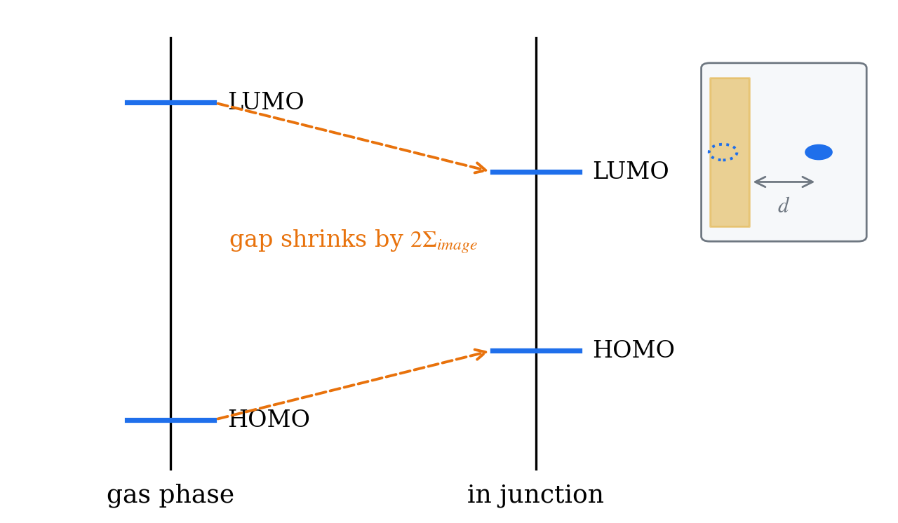
Figure 1. Level renormalization by electrode screening (image charge) — the gas-phase HOMO/LUMO gap is reduced inside the junction by $2\Sigma_{image}$. Inset: a charge in front of a metal surface and its mirror charge. (Schematic)

DFT+Σ, in the Quek–Neaton line of work, approximates the two physical effects above by two level shifts instead of a high-cost method like GW. It is a scissors correction that lowers occupied levels and raises unoccupied ones:

$$\Delta_{\mathrm{occ}} = \underbrace{\left(-\mathrm{IP} - \varepsilon_{\mathrm{HOMO}}^{\mathrm{DFT}}\right)}_{\Sigma^{1}:\ \text{gas-phase}} + \underbrace{W_{\mathrm{occ}}}_{\Sigma^{2}:\ \text{image charge}}, \qquad \Delta_{\mathrm{virt}} = \left(-\mathrm{EA} - \varepsilon_{\mathrm{LUMO}}^{\mathrm{DFT}}\right) + W_{\mathrm{virt}} .$$

Component (i): the gas-phase correction — the role of the VASP hybrid

Two routes to obtaining reference IP/EA values for the isolated molecule:

• ΔSCF — three total-energy calculations of the neutral, cationic, and anionic states. This is the literature standard, but it brings practical issues such as monopole corrections for charged cells under periodic boundaries and the choice of spin configuration for the charged states.
• Hybrid-functional eigenvalues — do a single-point calculation of the same isolated-molecule structure with B3LYP/HSE etc., and use the difference between the hybrid levels and the semi-local levels as the shift. This is a surrogate approximation to ΔSCF, and the VASP hybrid calculation prepared in Chapter 3 provides exactly this reference point.

Aligning references across codes

If the transport comes from SIESTA (LCAO) and the reference levels from VASP (plane-wave), the eigenvalues of the two codes must not be subtracted directly — code and basis offsets get mixed in with the functional difference. Compute a common functional (e.g. PBE) once more in each code as a bridge, and construct the terms so that subtraction always happens within the same code; the code offsets then cancel:

$$\Delta = \left[\varepsilon^{\mathrm{hybrid}} - \varepsilon^{\mathrm{PBE}}\right]_{\mathrm{VASP}} + \left[\varepsilon^{\mathrm{PBE}} - \varepsilon^{\mathrm{transport\ functional}}\right]_{\mathrm{SIESTA}} .$$

Component (ii): the image-charge correction

For planar metal electrodes this is estimated with the classical image-charge model. The stabilization energy of a point charge at distance $z$ from the electrode surface goes as $e^2/4(z-z_0)$ (with $z_0$ the image-plane position), and with two electrodes it extends to an infinite series sum. Occupied levels move up and unoccupied levels move down, narrowing the gap again — the opposite direction to component (i).

Implementation overview: injecting a projector ΔH via TBT.dH

If the correction is a static shift independent of energy, a self-energy correction is mathematically equivalent to a Hamiltonian correction. That is, without rerunning SIESTA, one simply adds $\Delta H$ to the $H$ that TBtrans uses to build the Green function:

$$G^r(E) = \left[(E + i\eta)S - (H + \Delta H) - \Sigma_L - \Sigma_R\right]^{-1}.$$

$\Delta H$ is built as a projector in the basis of the isolated-molecule MOs. With $C$ the matrix of PAO coefficients of the isolated-molecule MOs and $\Delta_i$ the per-orbital shifts,

$$\Delta H = S\, C\, \mathrm{diag}(\Delta_i)\, C^{\dagger}\, S$$

and constructing it this way shifts each MO in the generalized eigenvalue problem by exactly $\Delta_i$:

$$(H + \Delta H)\, c_j = (\varepsilon_j + \Delta_j)\, S\, c_j .$$

Points to watch in the implementation:

• In a non-orthogonal basis, $S$ must be sandwiched on both sides. The easy route of shifting only the diagonal onsite elements fails to move the levels by $\Delta$ and additionally distorts the orbital hybridization.
• $\Delta H$ acts only on the molecular (impurity) subspace. The electrode Hamiltonian and the lead self-energies are untouched.
• Save the completed $\Delta H$ in netCDF format (*.dH.nc) with sisl and inject it by specifying the path with the TBT.dH option in the TBtrans input (for the file format and the exact option spelling, check the TBtrans manual and the delta-file section of the sisl documentation).
• Since the correction enters only at the post-processing stage, the zero-bias TSHS is reused as is — no TranSIESTA reconvergence is needed.
• Two self-checks: ① transform $\Delta H$ back into the MO basis and confirm that $\mathrm{diag}(\Delta_i)$ is recovered; ② confirm that the first-order perturbation $\langle\psi_j|\Delta H|\psi_j\rangle$ agrees with the rediagonalized result.

One conceptual difficulty is worth noting. The "molecular subspace" is clear for a junction in which the molecule is weakly physisorbed to the electrodes, but for a case like our example (C19N), where the impurity is covalently fused into the chain, the definition itself is ambiguous. Cutting out a sub-block of the device Hamiltonian and diagonalizing it directly (the MPSH family of approaches) can give unphysical levels in a fused system, so the projector approach using the $C$ obtained from an isolated reference calculation is safer — though which atoms count as "the molecule" still remains the user's physical judgment.

Limits — using it honestly

DFT+Σ has a well-defined place on the ladder of approximations, and its quantitative validity collapses once its assumptions are violated.

1. The image-charge model is sensitive to electrode geometry. The standard planar formula presumes a flat metal surface and a well-defined image plane. For 1D chain electrodes like our example, no image plane is defined, and no published procedure extended to 1D geometry is established. In that case one applies only the gas-phase correction, omitting $\Sigma^2$; the gap opening is then an upper bound and the $T(E_F)$ suppression a lower-bound estimate.
2. The choice of ΔSCF reference matters. IP/EA depend on the spin configuration of the charged states, the vacuum-level alignment, and the periodic-cell corrections. Which reference was used must always be stated.
3. Assumptions: weak coupling and resonances far from $E_F$. The accuracy of the correction degrades as the molecule–electrode coupling grows stronger or as the resonances approach $E_F$ (Darancet 2012). A system with large charge transfer at the junction, where the frontier levels are pinned to $E_F$, undermines the assumptions themselves.
4. Non-self-consistent. Only the levels are moved; the charge density is not fed back.

The numbers of a corrected $T(E)$ are therefore safer interpreted as qualitative indicators at the level of "direction and order of magnitude of the correction", or as quantitative upper/lower bounds, rather than quoted directly.

Example flow: a conceptual exercise on C19N

The actual pipeline has five stages: ① isolated reference calculation (VASP hybrid or ΔSCF) → ② obtaining $\Delta_i$ → ③ extracting $C$ and assembling $\Delta H$ → ④ rerunning TBtrans with TBT.dH → ⑤ comparing $T(E)$ before and after the correction. Here we only run a toy model to get a feel for how the correction changes $T(E)$. In the tunneling region inside the gap, the transmission of a single resonance is approximated by a Lorentzian:

$$T(E) \approx \frac{\Gamma^2}{(E - \varepsilon_0)^2 + \Gamma^2}.$$

toy_scissors.py

import numpy as np
import matplotlib.pyplot as plt

E = np.linspace(-3, 3, 6001)          # eV, E - E_F
Gamma = 0.05                          # eV, electrode coupling width

def lorentz(E, eps0):
    return Gamma**2 / ((E - eps0)**2 + Gamma**2)

# before: occupied resonance just below E_F / after: lowered by 0.5 eV by the scissors shift
for eps0, label in ((-0.10, "before (PBE)"), (-0.60, "after (DFT+Sigma)")):
    plt.semilogy(E, lorentz(E, eps0), label=label)

plt.xlabel("E - E_F (eV)")
plt.ylabel("T(E)")
plt.legend()
plt.savefig("scissors_sketch.png", dpi=200, bbox_inches="tight")

Moving the resonance just 0.5 eV away from $E_F$ is enough to drop $T(E_F)$ by nearly two orders of magnitude. This is the substance of "level errors in PBE distort the conductance by orders of magnitude", and conversely it means that an uncertainty of a few hundred meV in the correction makes the $T(E_F)$ prediction equally uncertain.

Exercises

1. In the toy model, vary $\Gamma$ over 0.01, 0.05, and 0.2 eV and tabulate by what factor the same 0.5 eV shift changes $T(E_F)$. In which regime is the correction most dramatic?
2. In a two-level (HOMO/LUMO) model, apply corrections $\Delta_{\mathrm{occ}} < 0$ and $\Delta_{\mathrm{virt}} > 0$ and sketch, as a sum of two Lorentzians, how $T$ at the middle of the gap changes.
3. Build a non-orthogonal two-orbital model ($S_{12} \neq 0$) and compare the eigenvalue shifts obtained by raising only the onsite diagonal by $\Delta$ with those from using the $S C\,\mathrm{diag}(\Delta)\,C^{\dagger} S$ projector. This numerically confirms why $S$ is needed on both sides.
4. How would you define the "molecular subspace" in our C19N example? The single N atom only? N plus a few neighboring C atoms? Discuss how each choice would affect the projector correction.

References

• J. B. Neaton, M. S. Hybertsen, and S. G. Louie, "Renormalization of Molecular Electronic Levels at Metal-Molecule Interfaces", Phys. Rev. Lett. 97, 216405 (2006). DOI 10.1103/PhysRevLett.97.216405
• S. Y. Quek et al., "Amine-Gold Linked Single-Molecule Circuits: Experiment and Theory", Nano Lett. 7, 3477 (2007).
• P. Darancet et al., "Quantitative Current-Voltage Characteristics in Molecular Junctions from First Principles", Nano Lett. 12, 6250 (2012). DOI 10.1021/nl3033137