DFT Theory — From the Many-Body Problem to Kohn–Sham

Every electronic-structure calculation in this tutorial — from SIESTA's SCF (Chapter 01) to VASP relaxation (Chapter 03) and TranSIESTA transport — runs on density functional theory (DFT). This chapter lays that theoretical foundation. We work out why the many-body Schrödinger equation cannot be solved directly, what the Hohenberg–Kohn theorems guarantee, and how the Kohn–Sham construction turns that guarantee into a practical computational procedure. As a theory chapter, it contains no input-file or run sections.

Learning Objectives

• Explain why the dimensionality of the many-body wavefunction grows exponentially with the number of electrons, and state the content of the Born–Oppenheimer approximation.
• Grasp the statements and implications of the two Hohenberg–Kohn theorems — the density determines everything, and a variational principle holds.
• Understand the Kohn–Sham equations and the structure of the effective potential $v_{\mathrm{eff}} = v_{\mathrm{ext}} + v_H + v_{xc}$.
• Map each step of the self-consistency loop to the SCF keywords (dDmax, mixing) of the Chapter 01 hands-on.
• Distinguish, on the XC functional ladder (LDA → GGA → meta-GGA → hybrid), what each rung adds and at what cost.
• Outline the status of the KS eigenvalues and the origin of the band-gap underestimation problem.

1. The Many-Body Problem and Exponential Explosion

The non-relativistic Hamiltonian of a system of nuclei and electrons is known. Setting the nuclei aside for a moment and considering only $N$ electrons (in atomic units):

$$\hat H = -\frac{1}{2}\sum_{i=1}^{N} \nabla_i^2 + \sum_{i=1}^{N} v_{\mathrm{ext}}(\mathbf r_i) + \frac{1}{2}\sum_{i \neq j} \frac{1}{|\mathbf r_i - \mathbf r_j|}$$

The first term is the kinetic energy, the second the external potential created by the nuclei, and the third the electron–electron Coulomb repulsion. The equation itself is complete; the problem is that its solution, the many-body wavefunction $\Psi(\mathbf r_1, \ldots, \mathbf r_N)$, is a function of $3N$ variables. Even representing each coordinate axis with only 10 grid points, the number of values required is $10^{3N}$ — for a carbon chain of 8 atoms (48 electrons), that is $10^{144}$, impossible even to store.

The obvious attempt to escape the exponential explosion — writing $\Psi$ as a product of one-electron functions — is not exact because of the third term. The electron–electron interaction entangles the coordinates so that the variables do not separate, and this non-separability is correlation. The head-on route to the many-body problem is blocked; a detour is needed.

2. The Born–Oppenheimer Approximation

The first detour is the separation of nuclei and electrons. Nuclei are at least three orders of magnitude heavier than electrons (proton/electron mass ratio ≈ 1836). Assuming the electrons adapt instantaneously to the nuclear motion, we solve only the electronic problem with the nuclear coordinates held fixed — the nuclear positions $\{\mathbf R\}$ become parameters of the equation, not variables.

Obtaining the electronic ground-state energy for each nuclear configuration yields the potential energy surface $E(\{\mathbf R\})$, and its gradient gives the forces on the nuclei. Thanks to the Hellmann–Feynman theorem, these forces are computed directly from the converged electron density without differentiating the wavefunction with respect to the nuclear coordinates. This approximation is precisely why structural optimization (Chapter 03) is defined as "finding the nuclear configuration where the forces vanish." From here on, everything in this chapter is the electronic problem under fixed nuclei.

3. The Hohenberg–Kohn Theorems

The electronic problem is still $3N$-dimensional. Hohenberg and Kohn (1964) proved that a radical reduction is possible here. We state the two theorems without proof.

Theorem 1 (the density determines everything). The ground-state electron density $n(\mathbf r)$ uniquely determines the external potential $v_{\mathrm{ext}}(\mathbf r)$ (up to a constant). Since the potential fixes the Hamiltonian, which fixes the wavefunction and all observables, every ground-state property is, in principle, a functional of the density alone. This is an existence guarantee that $n(\mathbf r)$, a function of 3 variables, can serve as the fundamental variable in place of $\Psi$ with its $3N$ variables.

Theorem 2 (variational principle). There exists an energy functional $E[n] = F[n] + \int v_{\mathrm{ext}}(\mathbf r)\, n(\mathbf r)\, d\mathbf r$ such that $E[n] \geq E_0$ for any admissible density, with equality only at the true ground-state density. Here $F[n]$ is the universal functional containing the kinetic energy and the electron–electron interaction, taking the same form regardless of the system (regardless of what $v_{\mathrm{ext}}$ is).

Let us be clear about the meaning. The two theorems only guarantee that "the density suffices"; they do not reveal the concrete form of $F[n]$ — it is an existence proof, not a construction method. Knowing $F[n]$ exactly is as hard as solving the original many-body problem. DFT became a practical tool thanks to the Kohn–Sham construction of the next section.

4. The Kohn–Sham Construction — A Non-Interacting Auxiliary System

Kohn and Sham's (1965) idea is this. Introduce a fictitious non-interacting auxiliary system that has the same ground-state density as the real system. Since the kinetic energy of non-interacting electrons $T_s[n]$ and the classical Coulomb (Hartree) energy $E_H[n]$ can be computed exactly, the energy functional is decomposed as follows.

$$E[n] = T_s[n] + \int v_{\mathrm{ext}}\, n\, d\mathbf r + E_H[n] + E_{xc}[n]$$

The last term, $E_{xc}[n]$, is the exchange–correlation functional — defined as the "remainder" containing the difference between the true kinetic energy and $T_s$, plus all interaction effects beyond the classical Coulomb term. Exchange is the share coming from the antisymmetry of the wavefunction (the Pauli principle); correlation is everything beyond that. All the difficulty of the many-body problem has been quarantined into this single term, and it is the only unknown.

Applying the variational principle of Theorem 2 to this functional yields equations of one-electron form.

$$\left[-\frac{1}{2}\nabla^2 + v_{\mathrm{eff}}(\mathbf r)\right]\psi_i(\mathbf r) = \varepsilon_i\,\psi_i(\mathbf r), \qquad v_{\mathrm{eff}} = v_{\mathrm{ext}} + v_H + v_{xc}$$

These are the Kohn–Sham equations. $v_H = \delta E_H/\delta n$ is the classical Coulomb potential generated by the density, $v_{xc} = \delta E_{xc}/\delta n$ is the exchange–correlation potential, and the density is reconstructed from the occupied KS orbitals.

$$n(\mathbf r) = \sum_i^{\mathrm{occ}} |\psi_i(\mathbf r)|^2$$

The form is a one-electron Schrödinger equation, but since $v_{\mathrm{eff}}$ depends on the density, it is in substance a nonlinear problem. And from the moment $E_{xc}$ must be approximated, DFT becomes an approximate theory — which approximation to use is the subject of Section 6.

One point worth noting. The KS orbitals $\psi_i$ and eigenvalues $\varepsilon_i$ are, formally, auxiliary objects for constructing the density. Nevertheless, in practice band structures, DOS, and PDOS (Chapter 02) are all drawn from KS eigenvalues, and in most cases they reproduce the qualitative structure of experimental spectra well. Their quantitative status, however — especially the gap — has structural limitations, which is the subject of Section 7 and Chapter 11.

5. The Self-Consistency Loop

$v_{\mathrm{eff}}$ depends on $n$, and $n$ comes from the solutions $\psi_i$ of $v_{\mathrm{eff}}$. The solution is therefore a fixed point, found by iteration.

① Guess an initial density n⁰ (usually a superposition of neutral atomic densities)
② Construct v_eff[n]: compute the Hartree + XC potentials
③ Diagonalize the KS Hamiltonian → orbitals {ψ_i} and eigenvalues {ε_i}
④ Reconstruct a new density n_out from the occupied orbitals
⑤ Convergence test: is the difference between n_out and n_in below tolerance?
   Yes → done. Output total energy, forces, eigenvalues
   No  → ⑥ mixing: n_in(new) = a blend of n_in and n_out → return to ②

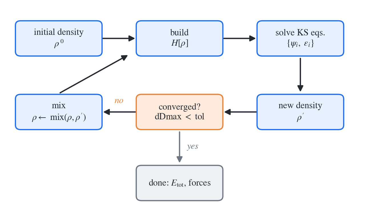
Figure 1. The self-consistency loop (schematic) — build $H[\rho]$ from the density, solve the KS equations to get a new density, and iterate with mixing until dDmax falls below tolerance.

The reason step ⑥ mixes in only part of $n_{\mathrm{out}}$ rather than using it wholesale as the next input is stability. In systems whose dielectric response diverges at long wavelengths, such as metals, a small change in density is amplified into a large change in potential (charge sloshing), and simple iteration oscillates or diverges. The standard prescription is to incorporate the new density gradually (linear mixing) and to estimate the optimal blend from the history of previous iterations (Pulay mixing).

Each step of this loop corresponds one-to-one with the keywords and outputs of the Chapter 01 hands-on.

Loop step	SIESTA keyword / output (Chapter 01)
① Initial density	DM.UseSaveDM — start from a saved density matrix if one exists (warm start)
③ Diagonalization	The main cost of one SCF iteration. The iscf counter is the iteration number
⑤ Convergence test	dDmax (maximum change of density-matrix elements between iterations) below SCF.DM.Tolerance
⑥ Mixing	SCF.Mixer.Weight 0.2 (blend in 20% of the new density), SCF.Mixer.History 15 (Pulay history)

Convergence failure appears in two forms. If dDmax oscillates without decreasing, the iteration map is unstable, and reducing the mixing weight is the first prescription — shrinking the step size of the iteration to stay within the stable region. Conversely, a calculation stopped by hitting MaxSCFIterations has not converged, and the judgment rule that its results must not be used (Chapter 01) also follows from this structure.

Eharris and E_KS — the two energy columns of the Chapter 01 output

Eharris and E_KS in the Chapter 01 stdout are two estimates of the same total energy. The Harris functional (Eharris) is evaluated from the input density of that iteration alone, while the Kohn–Sham functional (E_KS) is evaluated from the output density. Once the SCF converges and the input and output densities coincide, the two values merge into one. The shrinking difference between the two columns, together with dDmax, can therefore itself be read as a convergence indicator.

6. The XC Functional Ladder

What remains is the approximation of $E_{xc}[n]$. The approximations line up like a ladder according to how much information they use from the density.

Rung	Representatives	Input information	Character and cost
LDA	PZ, PW92	Local density $n(\mathbf r)$	Applies the homogeneous electron gas $\epsilon_{xc}(n)$ at each point. Remarkably robust, but tends to overbind (underestimates lattice constants)
GGA	PBE	$n$, $\nabla n$	Density-gradient correction. Greatly improves binding energies and structures at essentially the same cost as LDA. The de facto standard for solid-state calculations
meta-GGA	SCAN, etc.	$n$, $\nabla n$, kinetic-energy density $\tau$	Better discrimination of bonding types. Slightly higher cost, watch numerical stability
hybrid	B3LYP, HSE06, PBE0	+ a fraction of nonlocal HF exchange (usually 20–25%)	Mitigates self-interaction error, improves gaps and level positions. Nonlocal exchange raises the cost by one to two orders of magnitude

Perdew called this hierarchy "Jacob's ladder" — higher rungs are generally more accurate but costlier, and no rung beats the ones below on every problem. One practical rule follows: quantities to be compared must be computed with the same functional. Directly subtracting energies obtained at different rungs is meaningless.

This tutorial uses PBE as the standard, for two reasons. First, it is supported identically in both SIESTA and VASP, so the LCAO/plane-wave cross-validation (Chapter 03) and the entire transport workflow can be threaded through the same functional. Second, for structures, total energies, and forces, PBE is accurate enough for the cost.

Hybrids are far too expensive for full transport calculations and couple only in a limited way to LCAO NEGF implementations, so they are used only to produce the level reference of isolated molecules — that usage is the DFT+Σ correction of Chapter 11.

7. Band-Gap Underestimation — A Preview

One limitation should be known in advance. The KS eigenvalues $\varepsilon_i$ are Lagrange multipliers of the auxiliary system, not the energies of actually adding or removing electrons (quasiparticle energies). Semi-local functionals (LDA/GGA), due to self-interaction error and the missing derivative discontinuity, place occupied levels too high and unoccupied levels too low — as a result the band gap is systematically underestimated, with errors of tens of percent common in typical semiconductors.

For band shapes or structure prediction this is not a big problem, but in transport it can be fatal: if a resonant level's position is off by several hundred meV, $T(E_F)$ inside the gap is distorted by orders of magnitude. The origin of this error and the standard literature prescription (DFT+Σ) are covered in Chapter 11.

Key Takeaways

Concept	Content
Exponential explosion	$\Psi(\mathbf r_1,\ldots,\mathbf r_N)$ is $3N$-dimensional — direct solution impossible
Born–Oppenheimer	Fix the nuclei, solve only the electronic problem. $E(\{\mathbf R\})$ is the potential surface; its gradient gives the forces
HK Theorem 1	The ground-state density determines $v_{\mathrm{ext}}$ and all properties
HK Theorem 2	$E[n] \geq E_0$, equality at the true density — variational principle
KS construction	Non-interacting auxiliary system with the same density. $v_{\mathrm{eff}} = v_{\mathrm{ext}} + v_H + v_{xc}$
SCF loop	Density → potential → diagonalization → new density → mixing → convergence (dDmax, SCF.Mixer.*)
Eharris vs E_KS	Total energy evaluated from the input / output density — coincide at convergence
XC ladder	LDA → GGA (PBE) → meta-GGA → hybrid. This tutorial uses PBE + hybrid reference
KS gap	Not the quasiparticle gap — systematically underestimated with semi-local functionals (Chapter 11)

Exercises

1. A feel for the exponential explosion. Suppose the wavefunction is stored as a table with 10 grid points per coordinate axis. Estimate the storage required for 2 electrons (a He atom) and for 48 electrons (an 8-atom C chain), and compare with storing the density $n(\mathbf r)$ on the same grid.
2. The Hartree potential. Show that the functional derivative of $E_H[n] = \frac{1}{2}\iint \frac{n(\mathbf r)\,n(\mathbf r')}{|\mathbf r - \mathbf r'|}\, d\mathbf r\, d\mathbf r'$ is $v_H(\mathbf r) = \int \frac{n(\mathbf r')}{|\mathbf r - \mathbf r'|}\, d\mathbf r'$.
3. Why mixing is needed. Viewing the SCF iteration as fixed-point iteration of $n = g(n)$, the convergence condition is that the slope magnitude of the iteration map is less than 1. Explain why linear mixing $n^{(k+1)} = (1-\alpha)\,n^{(k)} + \alpha\, g(n^{(k)})$ can make a divergent iteration converge, and what you pay if $\alpha$ is reduced indiscriminately.
4. Harris vs KS energy. In the stdout of the Chapter 01 calculation, compare the difference between Eharris and E_KS at the first and last iterations. Explain, using the definitions of Section 5, why the two values approach each other as the iteration proceeds.
5. The meaning of KS eigenvalues. Based on Sections 6 and 7, summarize in two sentences why the observation that "the gap of a PBE band structure is smaller than experiment" is a structural limitation of the theory, not a calculation mistake. The numerical skeleton for actually solving the KS equations — basis expansion and k-sampling — continues in the next chapter — Bloch's Theorem and Basis Sets.

---

Ref: Hohenberg & Kohn, Phys. Rev. 136, B864 (1964); Kohn & Sham, Phys. Rev. 140, A1133 (1965); R. M. Martin, Electronic Structure: Basic Theory and Practical Methods (Cambridge University Press, 2004).