Bloch's Theorem and Basis Sets — Plane-Wave vs Localized Orbitals

To actually solve the Kohn–Sham equations established in DFT Theory, the orbitals $\psi_i$ must be expanded in a finite set of basis functions, turning the problem into a matrix eigenvalue problem. The choice of basis determines a code's character — VASP uses plane waves, SIESTA uses localized atomic orbitals (LCAO), and the reason this tutorial runs both codes in parallel is ultimately the division of labor between the strengths and weaknesses of the two bases. This chapter covers Bloch's theorem, the starting point for periodic systems; the structure and convergence parameters of the two bases; and the pseudopotential/PAW treatment of core electrons. As a theory chapter, it contains no input-file or run sections.

Learning Objectives

• Understand the statement of Bloch's theorem and the meaning of the band index $n$ and the crystal momentum $\mathbf k$.
• Explain the systematic convergence of the plane-wave basis (a single $E_{\mathrm{cut}}$) and its cost structure in vacuum-rich systems.
• Distinguish what norm-conserving pseudopotentials (SIESTA) and PAW (VASP) each freeze and each restore.
• Grasp the SZ/DZ/DZP hierarchy of the LCAO basis, the role of PAO.EnergyShift, and the pros and cons.
• Explain why NEGF transport presupposes a localized basis.

1. Periodic Potentials and Bloch's Theorem

A crystal is a system in which the same environment repeats under translation by any lattice vector $\mathbf R$: $V(\mathbf r + \mathbf R) = V(\mathbf r)$. Bloch's theorem states that this translational symmetry strongly constrains the form of the eigenstates.

$$\psi_{n\mathbf k}(\mathbf r) = e^{i\mathbf k \cdot \mathbf r}\, u_{n\mathbf k}(\mathbf r), \qquad u_{n\mathbf k}(\mathbf r + \mathbf R) = u_{n\mathbf k}(\mathbf r)$$

An eigenstate is a lattice-periodic function $u_{n\mathbf k}$ multiplied by a plane-wave phase, and it carries two labels. The crystal momentum $\mathbf k$ is the quantum number of translational symmetry, specifying the phase $e^{i\mathbf k \cdot \mathbf R}$ the wavefunction acquires when moving to a neighboring cell. The $\mathbf k$ values that give distinct physics are restricted to the first Brillouin zone (BZ). The band index $n$ enumerates the discrete eigenvalues obtained at fixed $\mathbf k$. Equivalently stated, a Bloch state acquires only a phase under lattice translation.

$$\psi_{n\mathbf k}(\mathbf r + \mathbf R) = e^{i\mathbf k \cdot \mathbf R}\, \psi_{n\mathbf k}(\mathbf r)$$

The problem of the infinite crystal has been decomposed into "the problem of a single unit cell × the $\mathbf k$ labels within the BZ," and connecting the eigenvalues as functions of $\mathbf k$, $\varepsilon_n(\mathbf k)$, gives the band structure. The 1D chain of this tutorial is periodic only along $z$, so the band structure is a one-variable function $\varepsilon_n(k_z)$ — the reason a single Γ–Z path suffices to draw all the bands in Chapter 02.

Enlarging the cell reduces the number of k-points needed. Stretching the real-space cell by a factor $m$ in one direction folds the BZ in that direction to $1/m$ (zone folding), and states originally scattered over several $\mathbf k$ collect inside the folded BZ. The practical rule "to keep the same k-space resolution, the number of divisions need only be inversely proportional to the cell length" comes from here; the general problem of representing the BZ by a finite set of $\mathbf k$ is covered in the next chapter.

2. The Plane-Wave Basis

Since $u_{n\mathbf k}$ is lattice-periodic, it expands exactly as a Fourier series over reciprocal lattice vectors $\mathbf G$.

$$\psi_{n\mathbf k}(\mathbf r) = \sum_{\mathbf G} c_{n\mathbf k}(\mathbf G)\; e^{i(\mathbf k + \mathbf G)\cdot \mathbf r}$$

The criterion for truncating the series is the kinetic-energy cutoff: $\frac{\hbar^2}{2m}|\mathbf k + \mathbf G|^2 \leq E_{\mathrm{cut}}$. This structure produces the strengths of the plane-wave basis.

• Systematic convergence — basis quality is controlled by one number, $E_{\mathrm{cut}}$, and raising it improves the result variationally and monotonically. VASP's ENCUT is exactly this value (Chapter 03).
• Origin independence — the basis is not attached to atoms but spread uniformly over the cell. Since the basis stays fixed as atoms move, there are no Pulay forces with respect to atomic positions, and the Hellmann–Feynman forces are exact as-is, an advantage for structural optimization.
• Uniform accuracy — every point in space is described at the same resolution. The basis has no bias.
• FFT efficiency — the kinetic energy is diagonal in reciprocal space and the potential in real space, so the Hamiltonian is applied quickly by shuttling between the two representations with FFTs.

The weakness is the flip side of uniformity. The number of basis functions is proportional to the cell volume $\Omega$.

$$N_{\mathrm{PW}} \approx \frac{\Omega}{6\pi^2}\left(\frac{2mE_{\mathrm{cut}}}{\hbar^2}\right)^{3/2}$$

This means vacuum is described at exactly the same cost as matter.

In a system like this tutorial's 1D chain, where a wide vacuum surrounds a handful of atoms, most of the cell is empty space yet the plane-wave count is set by the full cell volume, so the computational cost per atom becomes highly unfavorable. This is why a chain calculation with only a few atoms feels heavier than expected in Chapter 03 (Exercise 1 has you estimate the basis size directly). In practice $E_{\mathrm{cut}}$ is set at or above the PAW dataset's recommended value via a total-energy convergence test, and raised further in calculations where the cell varies, because of Pulay stress errors (Chapter 03).

3. Pseudopotentials and PAW — Treating Core Electrons

Plane waves come with one more cost problem. Core electrons (e.g., carbon 1s) are strongly localized near the nucleus, and valence wavefunctions also oscillate rapidly near the nucleus because of orthogonality to the core. Representing this sharp structure with plane waves would require an unmanageably large $E_{\mathrm{cut}}$. The standard prescription is two steps.

1. Frozen core — freeze the core electrons, which barely participate in chemical bonding, in their atomic states, and treat only the valence electrons explicitly.
2. Effective potential — replace the influence of the nucleus + core on the valence with an effective potential smoothed near the nucleus, constructed so that outside a certain radius it reproduces the same scattering properties as an all-electron calculation.

There are two implementation families, and the two codes use one each.

• Norm-conserving pseudopotentials — the pseudo-wavefunction is smooth and nodeless inside the core radius, but the charge (norm) inside is kept equal to that of the all-electron solution, securing the transferability of the scattering properties. This is what SIESTA uses; the .psml files handled in the hands-on are these pseudopotentials. The standard practice is not to generate them yourself but to obtain them from validated databases.
• PAW (projector augmented-wave) — maintains a linear transformation between the smooth pseudo-wavefunction and the all-electron wavefunction, so the true wavefunction near the nucleus can be restored when needed. It approaches all-electron accuracy with a smoother basis (lower cutoff) than norm-conserving schemes. VASP's POTCAR is the per-element PAW dataset.

Item	Norm-conserving (SIESTA)	PAW (VASP)
Data file	.psml	POTCAR
Construction principle	Conserves the charge (norm) inside the core radius	Maintains a pseudo ↔ all-electron linear transformation
Wavefunction near the nucleus	Only the pseudo form exists	All-electron form recoverable
Required cutoff	Relatively high	Low (smoother)

Either way, these approximations happen "off screen," so the practical rule for the user is to use validated datasets and respect the recommended cutoffs.

One corollary: when comparing two codes with different core treatments, like SIESTA (norm-conserving) and VASP (PAW), pseudopotential differences seep into the results alongside basis differences. Even with the same PBE, slight discrepancies in lattice constants are within the normal range, and absolute total energies have different reference points for each pseudopotential, so cross-code comparison of absolute energies is meaningless from the outset — compare only relative energies and structures/band shapes (see the SIESTA vs VASP comparison section of Chapter 03).

4. LCAO — A Numerical Atomic Orbital Basis

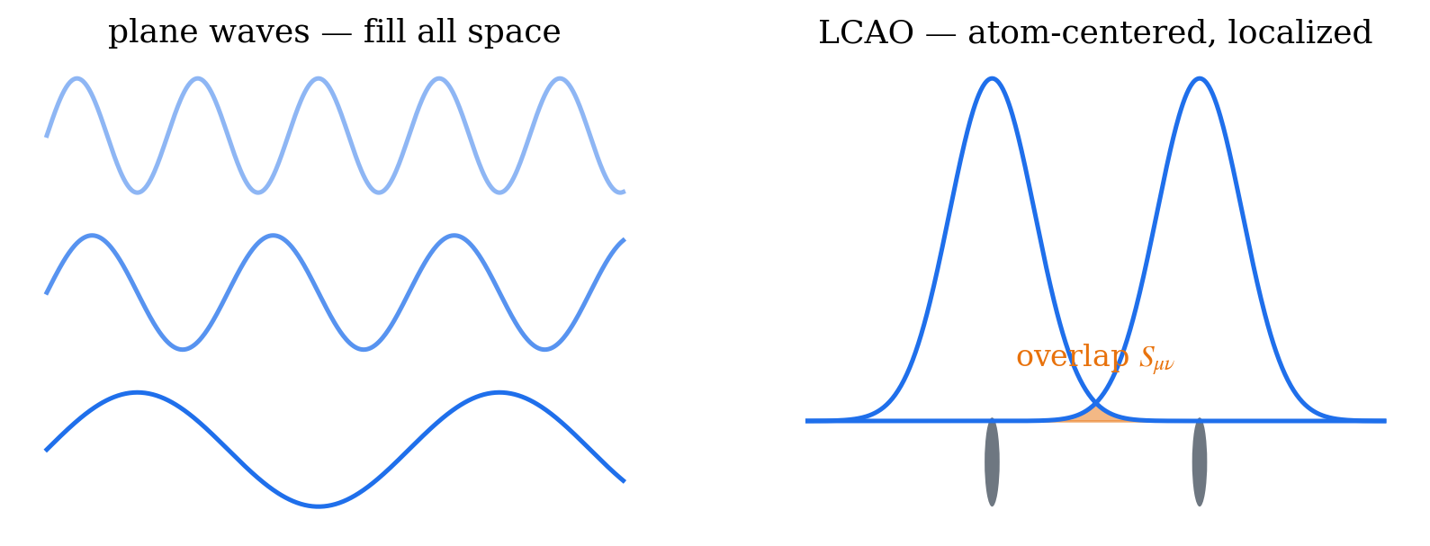
Figure 1. A plane-wave basis consists of sine waves filling all of space, while LCAO consists of localized orbitals centered on atoms — locality is what enables sparse matrices and spatial partitioning (transport). (Schematic)

SIESTA takes the opposite philosophy. Instead of spreading the basis uniformly over space, it attaches it to the atoms. It uses numerical atomic orbitals resembling each atom's valence orbitals, but confines them to be exactly zero beyond a specified radius (strictly confined). Basis quality is controlled along two axes.

• Number of radial functions (PAO.BasisSize) — SZ (1 radial function per valence orbital) → DZ (2) → DZP (2 + polarization orbitals). This hierarchy increases the orbitals' freedom to deform in a bonding environment; the standard in this tutorial is DZP (Chapter 01).
• Spatial extent of the orbitals (PAO.EnergyShift) — confining an orbital to a finite radius raises its energy slightly. PAO.EnergyShift specifies the allowed rise, and the smaller the value, the longer the orbital tail (larger radius). It is a device for setting the "range" of the basis consistently with a single energy criterion.

PAO.BasisSize    DZP        # SZ / DZ / DZP — radial-function hierarchy
PAO.EnergyShift  0.02 Ry    # smaller value → larger orbital radius

Taking carbon DZP as an example: 2 radial functions for $2s$ (2 orbitals) + 2 for $2p$ (6 orbitals) + 1 set of polarization $d$ (5 orbitals) = 13 orbitals per atom.

The advantages come from locality.

• Small matrices — with a dozen or so orbitals per atom (13 for carbon DZP), the matrix dimension is orders of magnitude smaller than the tens to hundreds of thousands of plane waves.
• Sparsity — since orbitals have finite range, Hamiltonian and overlap elements between distant atom pairs are exactly zero. Linear-scaling techniques for large calculations are built on this.
• Vacuum is cheap — the basis attaches only to atoms, so widening the vacuum does not grow the basis at all. In 1D chain + vacuum geometries, the cost structure is the exact opposite of plane waves.
• Spatial attribution — "this orbital belongs to this atom" is well defined, which is used directly in transport where region partitioning is required (Section 5). Atom-resolved decompositions such as PDOS and Mulliken analysis are likewise natural.

The disadvantages are also the flip side of locality.

• No systematic convergence — there is no single parameter that, like the plane-wave $E_{\mathrm{cut}}$, monotonically improves accuracy when turned up. Basis quality spans several axes — the SZ/DZ/DZP hierarchy, confinement radii — so judging "is it sufficiently converged?" is comparatively laborious.
• BSSE (basis set superposition error) — when two fragments approach, each borrows the other's basis functions, artificially overestimating the binding energy. This error must be managed, e.g., with counterpoise corrections, when comparing adsorption or binding energies.
• Limited description of diffuse states — the basis is confined to finite radii around atoms, so states extending far into the vacuum (vacuum tails of surface states, very diffuse unoccupied levels) are poorly represented.

The practical technique is to climb the hierarchy and check. Do quick exploration with SZ/DZ, production with DZP, and when in doubt, raise the basis one rung or reduce PAO.EnergyShift and see whether the results move — the SZ/DZ/DZP comparison in Chapter 01, Exercise 3 is the hands-on that builds this intuition.

MeshCutoff is not a basis parameter

MeshCutoff in the SIESTA input is unrelated to basis size. It sets the fineness of the real-space grid on which the electron density and potentials are represented; its name resembles the plane-wave code's ENCUT (basis size), making it easy to confuse, but its role is different. In SIESTA, basis quality is governed by PAO.BasisSize and grid integration accuracy by MeshCutoff. The eggbox effect — the energy rippling with atomic position when the grid is coarse — also comes from this grid, not the basis; it is measured directly in Chapter 01, Exercise 2.

5. Why NEGF Transport Requires a Localized Basis

The NEGF formalism of Chapter 04 starts by dividing the system into left electrode–device–right electrode and writing the Hamiltonian as a block tridiagonal matrix. For this partition to hold, each basis function must be spatially attributed to one of the three regions, the coupling between distant blocks must be exactly zero, and the semi-infinite electrodes must be treatable by unit-cell recursion (surface Green's functions). Finite-range LCAO satisfies all three conditions.

By contrast, plane waves spread over the whole cell satisfy none of them — the "ownership" of a basis function is undefined, and with periodic boundary conditions as their premise they cannot represent a semi-infinite boundary. This is the theoretical basis for this tutorial's division of labor — structural optimization and reference electronic structure with VASP (plane-wave), transport with SIESTA/TranSIESTA (LCAO).

Key Takeaways

Item	Plane-wave (VASP)	LCAO (SIESTA)
Convergence control	Single $E_{\mathrm{cut}}$ (ENCUT), variational and monotonic	SZ/DZ/DZP hierarchy + PAO.EnergyShift — multi-axis, less systematic
Typical convergence test	ENCUT scan	Basis-hierarchy scan (SZ → DZ → DZP → …)
Force calculation	No Pulay forces w.r.t. atomic positions	Basis attached to atoms, Pulay corrections needed (handled by the code)
Vacuum cost	Proportional to cell volume — vacuum costs the same	Proportional only to atom count — vacuum is free
Matrices	Large and dense (handled via FFT)	Small and sparse
Core treatment	PAW (POTCAR)	Norm-conserving pseudopotential (.psml)
BSSE	None	Present — beware in binding-energy comparisons
Atom-resolved decomposition (PDOS etc.)	Requires separate projection	Orbitals belong to atoms — natural
Transport (NEGF)	No spatial attribution — unsuitable	Block partitioning and surface Green's functions possible — the required basis

Exercises

1. Estimating the plane-wave count. For a cubic cell with side $20\ \text{Å}$ and $E_{\mathrm{cut}} = 500\ \mathrm{eV}$, estimate the basis size using $N_{\mathrm{PW}} \approx \frac{\Omega}{6\pi^2}(2mE_{\mathrm{cut}}/\hbar^2)^{3/2}$. Compare the order of magnitude with the LCAO basis size for describing 8 carbon atoms in the same cell with DZP (13 orbitals per atom).
2. Verifying the Bloch form. Given $\psi(\mathbf r) = e^{i\mathbf k \cdot \mathbf r} u(\mathbf r)$ with $u$ lattice-periodic, show that $\psi(\mathbf r + \mathbf R) = e^{i\mathbf k \cdot \mathbf R}\, \psi(\mathbf r)$ holds. This phase relation is the content of the statement "$\mathbf k$ is the quantum number of the translation operator."
3. Vacuum scaling. In a 1D chain calculation, discuss how the plane-wave basis size and the LCAO basis size each change when the $xy$ vacuum width is doubled, using the scalings of Sections 2 and 4.
4. The direction of PAO.EnergyShift. If PAO.EnergyShift is reduced (e.g., $0.02 \to 0.005\ \mathrm{Ry}$), work out in which direction each of the following moves: orbital radius, Hamiltonian sparsity, computational cost, and basis accuracy.
5. The direction of BSSE. Explain, using the variational principle, why BSSE always biases binding energies toward overestimation.
6. Designing a cross-code validation. The same structure was computed with SIESTA (DZP) and VASP (ENCUT 500 eV). Give two quantities that may be compared and two that must not be, with reasons based on the discussions of Sections 3 and 4. The other half of solving the KS problem in periodic systems — representing the BZ by a finite set of k-points and handling occupations in metals — is covered in the next chapter — Brillouin Zone Sampling and Smearing.

---

Ref: N. W. Ashcroft & N. D. Mermin, Solid State Physics, ch. 8; Soler et al., J. Phys.: Condens. Matter 14, 2745 (2002) — SIESTA method paper; Blöchl, Phys. Rev. B 50, 17953 (1994); Kresse & Joubert, Phys. Rev. B 59, 1758 (1999).