02. Band Structure and DOS

We add a band path and a PDOS block to the cumulene calculation of Chapter 01 and look into the electronic structure. There are two goals — to confirm from bands and DOS that the equidistant carbon chain is a metal, and to understand that this metallic state tends to transform, via the Peierls instability, into polyyne with bond length alternation (BLA). This physics is the foundation of the mini-project at the end of the tutorial (the polyyne–cumulene junction).

Learning objectives

• Define a 1D band path (Γ–Z) with BandLines/BandLinesScale
• Understand the structure of the siesta.bands file and plot it directly with python
• Compute DOS/PDOS with %block ProjectedDensityOfStates
• Read the metallicity of cumulene (half-filled π bands) from the bands and DOS
• Explain the relation between the Peierls instability and the polyyne gap

Background

The 1D Brillouin zone and the Γ–Z path

For a system periodic only along $z$, the Brillouin zone is the one-dimensional interval $k_z \in [-\pi/c, \pi/c]$. Thanks to time-reversal symmetry only half of it needs to be considered, and by convention the zone center is called Γ and the boundary $k_z = \pi/c$ is called Z. A single band path Γ–Z is sufficient — $x$ and $y$ are vacuum and carry no dispersion.

Why is cumulene a metal?

Of carbon's 4 valence electrons, 2 go into the sp-hybridized σ bonds along the chain, and the remaining 2 go into the doubly degenerate π bands formed by the two p orbitals perpendicular to the chain ($p_x$, $p_y$). In the equidistant chain these π bands are exactly half-filled. A half-filled band crosses the Fermi level, so cumulene is a metal.

One caveat — the true period of the equidistant chain is a single atom ($d = 1.29$ Å), but we are using a 4-atom cell ($c = 4d$). As the Brillouin zone shrinks to one quarter, the bands of the primitive cell fold in fourfold, and the Fermi crossing of the half-filled π bands appears near Γ of the folded zone. Even though there are more bands and they look complicated, the physics is the same.

The Peierls instability — the road to polyyne

A 1D metal is intrinsically unstable against lattice distortion (Peierls' theorem). If the chain dimerizes — if the bonds alternate between short and long (bond length alternation, BLA) — a gap opens at the Fermi crossing, the occupied states are lowered in energy, and the total electronic energy gains. In the carbon chain this distorted phase is polyyne (alternating single and triple bonds, e.g., 1.34/1.24 Å), a semiconductor with an open gap.

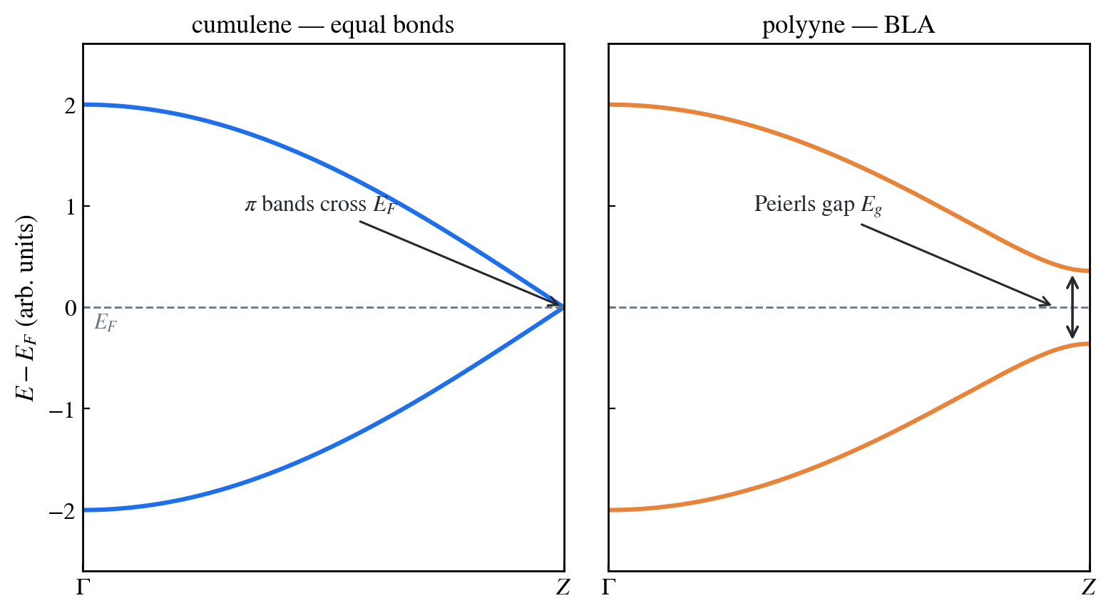
Figure 1. Band sketch of the Peierls instability (tight-binding schematic) — equidistant cumulene is a metal whose $\pi$ bands cross $E_F$ at the zone boundary, and once BLA sets in, a gap $E_g$ opens at that point.

That is, a chain of the same atoms at the same density switches between metal (cumulene) and semiconductor (polyyne) purely through the arrangement of bond lengths. This contrast is revisited in the mini-project, where a junction of the two phases is built and examined with transport.

DOS and PDOS

The density of states is defined as

$$D(E) = \sum_{n\mathbf{k}} \delta(E - \epsilon_{n\mathbf{k}})$$

and in practical calculations it is obtained by replacing the δ function with a Gaussian of finite width (broadening). The PDOS (projected DOS) decomposes this into atomic and orbital components, answering "which orbitals do the states near the Fermi level come from?" For cumulene, one sees that the region near $E_F$ is dominated by the C $p$ component (the π bands).

Input file

Keep the input.fdf of Chapter 01 as is and append the blocks below at the end of the file (system, basis, and k-grid settings are identical — the same system is reused). The complete file is in the example repository at code/ch02-bands.

input.fdf (appended blocks)

# --- band structure: Gamma-Z ---
BandLinesScale ReciprocalLatticeVectors
%block BandLines
  1   0.000  0.000  0.000  \Gamma
 60   0.000  0.000  0.500  Z
%endblock BandLines

WriteEigenvalues T

# --- DOS / PDOS ---
%block ProjectedDensityOfStates
  -20.00  10.00  0.100  2000  eV
%endblock ProjectedDensityOfStates

%block PDOS.kgrid_Monkhorst_Pack
   1   0   0    0.0
   0   1   0    0.0
   0   0 128    0.0
%endblock PDOS.kgrid_Monkhorst_Pack

Line-by-line commentary

• BandLinesScale ReciprocalLatticeVectors — interpret the k coordinates in BandLines as fractions of the reciprocal lattice vectors. $(0, 0, 0.5)$ is then Z ($k_z = \pi/c$).
• %block BandLines — each line is number of points, 3 k coordinates, label. The 1 on the first line marks the starting point of the path, and the 60 on the second line means the segment from Γ to Z is traced with 60 points. The label \Gamma is written verbatim into the siesta.bands file and used by plotting tools as the tick name.
• WriteEigenvalues T — write the eigenvalues at the SCF-sampled k-points to the output.
• %block ProjectedDensityOfStates — the order is Emin Emax broadening npoints unit. The window from $-20$ eV to $+10$ eV is computed with 0.1 eV Gaussian broadening at 2000 energy points. The energies are on an absolute scale (same reference as the eigenvalues), not relative to the Fermi level, so subtract $E_F$ when plotting.
• %block PDOS.kgrid_Monkhorst_Pack — a k-grid dedicated to the PDOS. The DOS is more sensitive to k-convergence than the bands, so a denser 128 is specified separately from the SCF grid (64).

Running

Same as Chapter 01.

siesta < input.fdf > siesta.out

After the SCF converges, the band-path calculation and the PDOS calculation follow, and siesta.bands and siesta.PDOS (XML format) are additionally generated. If you run in a directory where the siesta.DM of Chapter 01 remains, the SCF finishes in just a few iterations thanks to DM.UseSaveDM T.

Analyzing the output

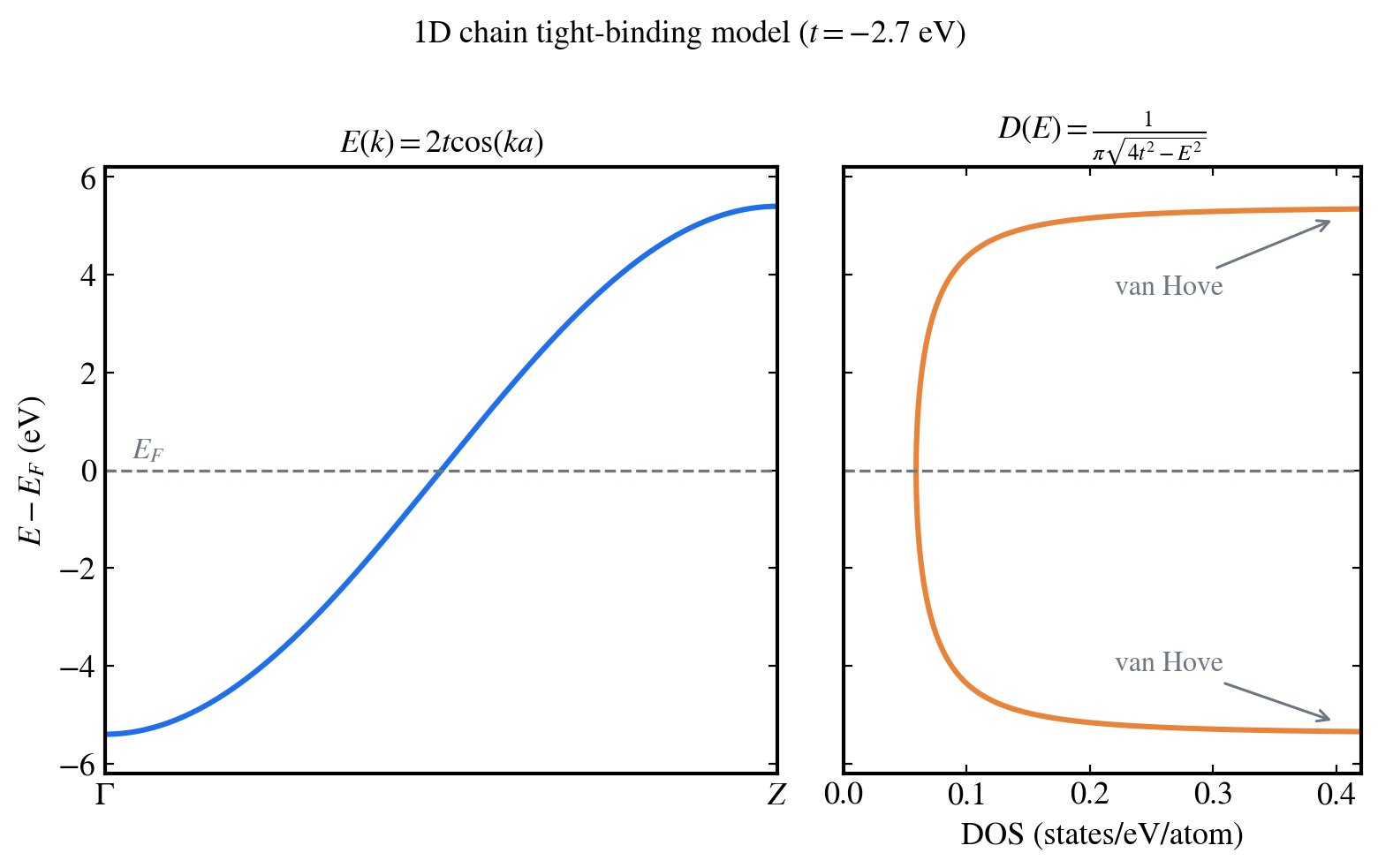
Figure 2. Bands and DOS of a 1D chain computed with a TB model — the qualitative form of the result the SIESTA calculation of this chapter gives. A van Hove peak of the DOS stands at every band edge. (Actual TB-model calculation, _scripts/fig_examples_batch.py)

Structure of the siesta.bands file

siesta.bands is a text file with a fixed structure.

   -4.591428                      # line 1: Fermi energy (eV)
    0.000000    0.322190          # line 2: path coordinate min/max
  -24.376912     8.914327         # line 3: eigenvalue min/max (eV)
   52    1   61                   # line 4: number of bands, spins, k-points
    0.000000  -24.376912  -24.301523  ...   # then: k coordinate + eigenvalues
    ...                                     # (eigenvalues of one k-point wrap over multiple lines)
   2                              # end: number of labels
    0.000000  '\Gamma'
    0.322190  'Z'

• Reading the Fermi energy from the first line and shifting the axis to $E - E_F$ is the first step of any plot.
• The 52 bands come from 4 atoms × 13 DZP orbitals.
• The k-coordinate column is the accumulated distance along the path. The absolute unit does not matter for the plot — just attach the Γ and Z labels at the two endpoints.

Plotting bands with python

Even though the eigenvalues wrap over multiple lines, reading token by token keeps the parser simple.

import numpy as np
import matplotlib.pyplot as plt

tokens = open("siesta.bands").read().split()
it = iter(tokens)

ef = float(next(it))                                  # Fermi energy
kmin, kmax = float(next(it)), float(next(it))
emin, emax = float(next(it)), float(next(it))
nb, ns, nk = int(next(it)), int(next(it)), int(next(it))

k = np.empty(nk)
E = np.empty((nk, nb * ns))
for ik in range(nk):
    k[ik] = float(next(it))
    E[ik] = [float(next(it)) for _ in range(nb * ns)]

plt.figure(figsize=(4, 6))
plt.plot(k, E - ef, color="C0", lw=1.2)
plt.axhline(0.0, color="k", ls="--", lw=0.8)
plt.xticks([k[0], k[-1]], [r"$\Gamma$", "Z"])
plt.xlim(k[0], k[-1])
plt.ylim(-10, 10)
plt.ylabel(r"$E - E_F$ (eV)")
plt.tight_layout()
plt.savefig("bands.png", dpi=300)

With sisl it is even shorter — sisl.get_sile("siesta.bands") gives a file object from which the data can be read. However, since the purpose of this chapter is to understand the file structure directly, the manual parser is the default.

Interpreting the bands

What to check in the plot:

• There are bands crossing $E_F$ (0 eV in the figure) — it is a metal.
• The bands near the Fermi crossing are doubly degenerate (the degeneracy of the $p_x$, $p_y$ π bands). The two bands overlap exactly and appear as a single line, but checking the eigenvalues in the file shows the same value appearing twice.
• Because the 4-atom cell was used, the bands are folded in. As explained in the background section, the crossing of the half-filled π bands appears near Γ of the folded zone.

PDOS

siesta.PDOS is in XML format, recording the projection of each orbital as a function of energy. It can be read with sisl and summed over any desired orbital combination; if only the total DOS is needed, the sum of all projections is the total DOS. There is one piece of physics to verify — the DOS at $E_F$ is finite (metal), and its component comes from the C $p$ orbitals (the π bands).

Exercises

1. Polyyne bands — change only the atomic coordinates as below (bond alternation 1.24/1.34 Å, cell length kept at 5.16 Å), repeat the same calculation, and overlay the bands. Confirm that the Fermi crossing near Γ disappears and a gap opens. Read the gap size (eV) from the bands, and compare whether the total energy has become lower than cumulene (by how many meV per atom).

   %block AtomicCoordinatesAndAtomicSpecies
      7.500000   7.500000   0.000000  1
      7.500000   7.500000   1.240000  1
      7.500000   7.500000   2.580000  1
      7.500000   7.500000   3.820000  1
   %endblock AtomicCoordinatesAndAtomicSpecies

2. Verifying folding — recompute cumulene with the single-atom primitive cell ($c = 1.29$ Å, k-grid $1 \times 1 \times 256$) and plot the bands. Check whether the bands of the 4-atom cell match the primitive bands folded fourfold, and where the Fermi crossing sits in the primitive zone ($k_z = \pi/2d$).

3. Effect of broadening — vary the PDOS broadening over 0.05, 0.1, 0.3 eV and overlay the DOS. Observe that with large broadening the van Hove singularities characteristic of 1D systems (the sharp peaks at band edges) are smeared out.

Having seen that the structure changes the energies and bands, the next chapter deals with how that structure itself is determined — Chapter 03 — Structure Optimization with VASP.