Brillouin Zone Sampling and Smearing

In the previous chapter we saw that eigenstates of a periodic system carry a $\mathbf k$ label. Physical quantities such as the electron density and total energy are defined as integrals over the entire Brillouin zone (BZ), yet an actual calculation can only approximate them as sums over a finite number of $\mathbf k$-points. This chapter covers the standard tools of that approximation — the Monkhorst–Pack grid, symmetry reduction, and the smearing that becomes essential for metals — and establishes the practical rules for designing k-grids according to dimensionality (3D/2D/1D) and material type (metal/insulator). As a theory chapter, it contains no input-file or run sections.

Learning Objectives

• Understand the procedure that converts a BZ integral into a weighted sum over a finite k-grid, and the structure of the Monkhorst–Pack grid.
• Explain why a single k-point suffices along vacuum directions, and the rationale for this tutorial's $1 \times 1 \times 64$ grid.
• Explain why k-convergence of metals is slower than that of insulators, in terms of the discontinuous occupation at the Fermi surface.
• Distinguish the characteristics and uses of the four smearing schemes (Fermi–Dirac, Gaussian, Methfessel–Paxton, tetrahedron).
• Understand that smearing is a convergence aid and that the free energy must be distinguished from $E(\sigma \to 0)$.

1. From BZ Integrals to Finite k-Grid Sums

The electron density of a periodic system is a double sum/integral over bands and the BZ.

$$n(\mathbf r) = \sum_n \int_{\mathrm{BZ}} \frac{d\mathbf k}{\Omega_{\mathrm{BZ}}}\; f_{n\mathbf k}\, |\psi_{n\mathbf k}(\mathbf r)|^2 \;\;\longrightarrow\;\; \sum_n \sum_{\mathbf k} w_{\mathbf k}\, f_{n\mathbf k}\, |\psi_{n\mathbf k}(\mathbf r)|^2$$

Replacing the integral with a finite sum carrying weights $w_{\mathbf k}$ is k-sampling. The standard is the Monkhorst–Pack (MP) grid — a uniform grid dividing the BZ into $N_1 \times N_2 \times N_3$ parts along each reciprocal-lattice direction. Written in one dimension, the grid points of an $N$-division grid are:

$$k_i = \frac{2i - N - 1}{2N}\,\frac{2\pi}{a}, \qquad i = 1, \ldots, N$$

In the original definition, the grid-point positions depend on whether the division count is odd or even. An odd division includes the Γ point ($\mathbf k = 0$); an even division shifts the grid by half a step and does not include Γ. A Γ-centered grid is a variant aligned so that Γ is always included regardless of the division count. In most cases the two converge similarly, but for hexagonal lattices a shifted even MP grid can produce a k-set inconsistent with the crystal symmetry, so using Γ-centered is the safe standard.

Not all k-points of a uniform grid are independent. Grouping points equivalent under time-reversal symmetry ($\varepsilon_n(\mathbf k) = \varepsilon_n(-\mathbf k)$) and the crystal point group leaves only the set of representative points — the irreducible BZ (IBZ) — with weights $w_{\mathbf k}$ proportional to each representative's multiplicity. The code does this automatically, and in high-symmetry systems the number of k-points actually computed shrinks to a fraction of the nominal grid. In SIESTA this grid is specified by %block kgrid_Monkhorst_Pack, in VASP by the KPOINTS file.

The yardstick for choosing the division count is its product with the real-space cell length. As seen in the zone folding of the previous chapter, stretching the cell by $m$ folds the BZ to $1/m$, so keeping $N_i \times a_i$ (division count × cell edge length) constant preserves the k-space resolution. If a system needed $1 \times 1 \times 64$ in the unit cell, an 8× supercell of the same material achieves the same resolution with $1 \times 1 \times 8$.

2. Rules by Dimensionality — The Grid Shape Follows the System's Periodicity

k-sampling is meaningful only along periodic directions. Along directions separated by vacuum, the wavefunctions of neighboring images do not overlap, so the bands have no dispersion in that direction (they are flat), and any $\mathbf k$ gives the same value — sampling several points merely repeats the same calculation. The grid shape therefore mirrors the system's dimensionality directly.

System	Grid shape	Rationale
3D bulk	$N \times N \times N$ (adjusted inversely to cell edge lengths)	All three directions periodic
2D slab	$N \times N \times 1$	Direction normal to the surface is vacuum — no dispersion
1D chain	$1 \times 1 \times N$	Only the chain axis is periodic; $xy$ is vacuum

This tutorial's $1 \times 1 \times 64$ (Chapter 01) is exactly the third row. The $xy$ vacuum directions get a single Γ point, and only the periodic $z$ direction is densely sampled with 64 points. Why 64 points are needed along $z$ is the subject of the next section — because this chain is a metal.

The k-convergence of metals and insulators differs qualitatively. In insulators and semiconductors every band is either completely filled or completely empty, so the integrand is smooth in $\mathbf k$ and converges quickly (essentially exponentially) with few k-points. In metals the Fermi surface cuts through the BZ and the occupation switches discontinuously from 1 to 0, so the discontinuity of the integrand must be resolved by the finite grid, making convergence slow. In a 1D metallic chain, the Fermi "surface" collapses to a Fermi point, making sampling near it especially sensitive — verified directly in the k-convergence test of Chapter 01, Exercise 1.

Two distinctions are worth recording together. First, the k-path of a band-structure calculation is separate from the SCF grid — the SCF converges the density with a uniform grid representing the whole BZ, and the bands then compute eigenvalues only along a high-symmetry line path on top of that converged density (Chapter 02). Second, in the transport workflow the electrode calculation's k-grid carries a separate constraint of matching the device calculation (Chapter 05), and specifying TBtrans's k-grid has a placement-rule pitfall (Chapter 07, Pitfall 2).

3. Smearing — Why It Is Needed

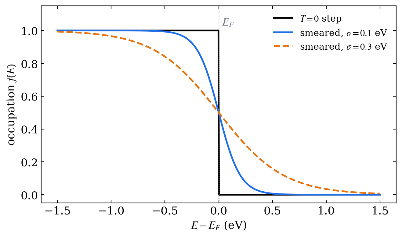
Figure 1. The $T=0$ step occupation function (black) and smeared occupations (blue, orange) — a larger smearing width $\sigma$ softens the discontinuity at the Fermi surface so the k-integral converges faster, but physical quantities must be judged by extrapolating $\sigma\to0$. (Schematic)

The root cause of the slow k-convergence of metals is that the $T = 0$ occupation function is a step: $f_{n\mathbf k} = \theta(E_F - \varepsilon_{n\mathbf k})$. On a finite grid, every time a k-point is added or moved, some state crosses the Fermi level and its occupation jumps discontinuously between 0 and 1, and the total energy fluctuates with the grid. The prescription is to replace the occupation by a smooth function of width $\sigma$.

$$f_{n\mathbf k} = f\!\left(\frac{\varepsilon_{n\mathbf k} - \mu}{\sigma}\right)$$

With smooth occupations the integrand also becomes smooth, and stable values emerge even from coarse grids. The price is that the result now depends on $\sigma$.

Another point to note is variational consistency. The quantity variationally consistent with smooth occupations is not the internal energy $E$ but the free energy, which includes a generalized entropy term.

$$F = E - \sigma\, S[f]$$

Forces and stresses must also be computed as derivatives of $F$ to agree with the energy change upon moving atoms. This is why the codes print the free energy separately — the FreeEng column in the SIESTA stdout (Chapter 01), and F in the VASP OSZICAR (Chapter 03). The difference between $F$ and $E$ widens as $\sigma$ grows, so its magnitude is itself the gauge of smearing contamination.

4. Smearing Schemes and Their Characteristics

Method	Occupation function	Characteristics	VASP	SIESTA
Fermi–Dirac	$[1 + e^{x}]^{-1}$	The thermal occupation of a physical electronic temperature $T = \sigma/k_B$ as-is — the only scheme where $\sigma$ has a physical interpretation. Long tails mean larger contamination at the same $\sigma$	ISMEAR = -1	OccupationFunction FD + ElectronicTemperature
Gaussian	erf-based	Safe general-purpose choice. A safe default for systems not yet classified metal/semiconductor and for relaxations	ISMEAR = 0	—
Methfessel–Paxton	Hermite polynomial corrections	Suppresses the $\sigma$ dependence of $E$ to higher order — the standard for metal relaxations. Occupations can go negative or exceed 1 (unphysical), so beware in analyses that interpret occupations	ISMEAR = 1, 2	OccupationFunction MP
tetrahedron (+Blöchl corrections)	Not an occupation function — divides the BZ into tetrahedra and integrates by linear interpolation	No smearing parameter at all. Optimal for precise total energies and DOS. Forces/stresses lack variational consistency, so unsuitable for relaxations; requires a minimum number of k-points	ISMEAR = -5	Not supported

The parameter correspondence between the two codes differs only in units. VASP specifies SIGMA directly in eV, while SIESTA specifies ElectronicTemperature as a temperature (or in energy units), converted via $\sigma = k_B T$. $300\ \mathrm{K} \approx 25.9\ \mathrm{meV}$, and Chapter 03's SIGMA = 0.05 eV corresponds to about $580\ \mathrm{K}$. If no occupation function is specified, SIESTA uses Fermi–Dirac.

SIESTA's default smearing

SIESTA's default is OccupationFunction FD + ElectronicTemperature 300 K, i.e., Fermi–Dirac smearing with $\sigma \approx 25.9\ \mathrm{meV}$. The Chapter 01 calculation, which specifies nothing, also runs with this setting, and this entropy term is why the FreeEng column in the stdout differs slightly from the total energy.

Negative occupations of Methfessel–Paxton

MP smearing allows negative regions in the occupation function for the sake of energy accuracy. Total energies and forces are unaffected, but analyses that read occupation numbers as physical quantities (partial charges, magnetization decompositions, etc.) can pick up artificial values. A classic pitfall is applying MP with a large $\sigma$ to a gapped system, putting negative occupations on states at the gap edges — for systems that might turn out to be semiconductors, Gaussian is the safe choice.

5. Practical Rules

Choice by purpose.

• Relaxation of a definite metal — Methfessel–Paxton + small $\sigma$ (0.05–0.2 eV). The stable forces provided by smooth occupations are what matter.
• Before metal/semiconductor classification, or relaxations in general — Gaussian + small $\sigma$. Chapter 03's ISMEAR = 0, SIGMA = 0.05 is this rule applied.
• Precise total energy and DOS at fixed structure — if the code supports it, tetrahedron (+Blöchl corrections) is best. There is no smearing contamination at all. But do not use it for relaxations.
• Finite-temperature properties, occupations of NEGF electrodes — Fermi–Dirac. The only case where $\sigma$ is a physical parameter (see below).

Also remember that calculations examining spectral shape, such as DOS, require a denser k-grid than total energies — total energies are integrals so errors cancel, whereas DOS must be resolved energy by energy.

Smearing is a convergence aid, not a physical parameter. The answer we want is the $T = 0$ energy in the limit $\sigma \to 0$ with an infinitely dense k-grid. $\sigma$ is merely a numerical device for approaching that limit with a finite grid; increasing $\sigma$ speeds up k-convergence but contaminates the answer itself — the two parameters must be checked together. The one exception is Fermi–Dirac: only when the thermal occupation of an actual electronic temperature is inserted deliberately (e.g., finite-temperature properties, the Fermi function of NEGF electrodes) does $\sigma$ become a physical parameter.

Gauge the size of the contamination by the difference between $F$ and $E$ from Section 3, and remove it if necessary by $\sigma \to 0$ extrapolation. For Gaussian smearing the extrapolation relation $E(\sigma \to 0) \approx (F + E)/2$ holds, and E0 in the VASP OSZICAR is exactly this extrapolated value — this is the basis for Chapter 03's rule that "energy comparisons between structures use E0." If the difference between $F$ and $E$ is non-negligible, that signals $\sigma$ is too large.

k-convergence test procedure. Always perform it once for a new system.

1. Fix all other parameters — basis, cutoff, etc.
2. Vary only the division count along the periodic direction through an increasing sequence (e.g., $k_z$ = 16, 32, 64, 128 in 1D) and compute the total energy.
3. Tabulate the total energy per atom, and adopt the smallest grid for which the difference between two adjacent settings falls below the target threshold (conventionally 1 meV per atom).
4. For a metal, repeat the same table at two values of $\sigma$ (e.g., the standard value and half of it) and confirm the adopted grid is insensitive to the choice of $\sigma$.

The template for the summary table is as follows (fill the values with your own calculations).

$k_z$	$E$ (eV/atom)	Diff. vs previous (meV/atom)	Verdict
16	…	—
32	…	…
64	…	below 1	adopt
128	…	…	check

If the calculation compares energy differences (binding energies, relative stabilities), then having the compared cases use the same grid and same smearing comes before absolute convergence — an arrangement that preserves error cancellation. The hands-on for this procedure is Chapter 01, Exercise 1.

Key Takeaways

Concept	Content
BZ integral	$\int_{\mathrm{BZ}} d\mathbf k \to \sum_{\mathbf k} w_{\mathbf k}$ — uniform MP grid + IBZ symmetry reduction
Γ-centered	Always includes Γ. An essential choice for hexagonal cells
Grid density yardstick	Keep $N_i \times a_i$ constant — as the cell grows, reduce the division count inversely
Grid shape	Sample only periodic directions — $N^3$ for 3D, $N \times N \times 1$ for slabs, $1 \times 1 \times N$ for 1D chains
Metal vs insulator	Insulators converge fast; metals converge slowly due to the Fermi-surface discontinuity — dense grid + smearing
Smearing	Softens the step occupation with width $\sigma$. The variationally consistent quantity is $F = E - \sigma S$
Schemes	FD (physical temperature), Gaussian (general-purpose), MP (metal relaxations, beware negative occupations), tetrahedron (precise energies/DOS, unsuitable for relaxations)
Code correspondence	VASP ISMEAR/SIGMA ↔ SIESTA OccupationFunction/ElectronicTemperature ($\sigma = k_B T$)
Principle	Smearing is a convergence aid — the goal is the $\sigma \to 0$ limit. E0 = the Gaussian extrapolated value

Exercises

1. k-convergence of a 1D toy model. For the 1D tight-binding band $\varepsilon(k) = -2t\cos(ka)$ at half-filling ($E_F = 0$), write code that computes the band energy $\frac{a}{\pi}\int_0^{\pi/a} \varepsilon(k)\, f(\varepsilon(k))\, dk$ as a uniform k-grid sum. Compare the convergence rate as the grid count increases for $\sigma = 0$ (step occupation) and Gaussian smearing ($\sigma = 0.1t$).
2. Whether Γ is included. Confirm from the MP grid-point formula of Section 1 that $k = 0$ is included only when $N$ is odd, and sketch how the point placement differs from a Γ-centered grid for an even-$N$ example.
3. $\sigma$ extrapolation. Suppose a metal calculation yields $F$ and $E$ for $\sigma$ = 0.05, 0.1, 0.2 eV. Based on the structure $F = E - \sigma S$ from Section 3, explain why $F$ and $E$ must converge to the same value as $\sigma \to 0$ and why $(F+E)/2$ is a good extrapolation.
4. Unit conversion. What electronic temperature in K does SIGMA = 0.2 eV correspond to? Conversely, how many meV is $k_B T$ at room temperature (300 K)? From this comparison, confirm that the smearing widths used in relaxations mostly correspond to fictitious temperatures far above actual experimental temperatures.
5. Grid design. If a $12^3$ grid was appropriate for a 3D metallic bulk with a cubic cell of side 4 Å, what grid would you propose for a slab of the same material (same in-plane cell, 20 Å vacuum in the normal direction)? Also discuss whether using multiple k-points along the vacuum direction changes anything in the results beyond being wasteful. This concludes the theoretical preparation of Fundamentals. The conceptual skeleton of how current flows in nanoscale devices — Chapter 00 — Overview of Quantum Transport — begins the main part.

---

Ref: Monkhorst & Pack, Phys. Rev. B 13, 5188 (1976); Methfessel & Paxton, Phys. Rev. B 40, 3616 (1989); Blöchl, Jepsen & Andersen, Phys. Rev. B 49, 16223 (1994).