04. The NEGF Formalism — Green's Functions and Self-Energy

In Chapter 00 we saw that the current is determined by the transmission function $T(E)$. This chapter establishes the framework for computing $T(E)$ from a first-principles Hamiltonian — the non-equilibrium Green's function (NEGF) formalism. We work out how an open quantum system is turned into a finite matrix problem, what the self-energy and broadening are, and which parts of the formalism TranSIESTA and TBtrans each handle. Since this is a theory chapter, there are no input files or run sections.

Learning objectives

• Understand the block structure of the Hamiltonian of an open quantum system partitioned into left electrode–device–right electrode.
• Explain why NEGF requires a local-orbital (LCAO) basis rather than plane waves.
• Grasp the physical meaning of the retarded Green's function $G(E)$, the self-energies $\Sigma_{L,R}$, and the broadenings $\Gamma_{L,R}$.
• Learn the Caroli/Landauer formula $T(E) = \mathrm{Tr}[\Gamma_L G \Gamma_R G^\dagger]$ and the spectral function–DOS relation.
• Distinguish the division of labor between TranSIESTA (self-consistent NEGF) and TBtrans (post-processing transport).

1. Open quantum systems and spatial partitioning

The stage for the transport problem is not a closed periodic system but an open system. We divide the system into three regions.

• Left electrode (L) — a periodic conductor extending semi-infinitely along the transport direction ($z$)
• Device (D) — the central region where scattering occurs (the scattering region). Atomic arrangements different from the electrodes, defects, molecules, etc. go here
• Right electrode (R) — the semi-infinite conductor on the opposite side

If the basis functions are spatially localized, the Hamiltonian has a block tridiagonal structure.

$$H = \begin{pmatrix} H_L & V_{LD} & 0 \\ V_{LD}^\dagger & H_D & V_{DR} \\ 0 & V_{DR}^\dagger & H_R \end{pmatrix}$$

The key assumption is that the block directly connecting L and R is zero — the device must be long enough that the two electrodes do not overlap directly. The overlap matrix $S$ has the same block structure (LCAO bases are not orthogonal, so $S \neq I$).

The full matrix is infinite-dimensional, but all we want are physical quantities of the device block. The essence of NEGF is to fold the effect of the semi-infinite electrodes into a self-energy on the finite device block.

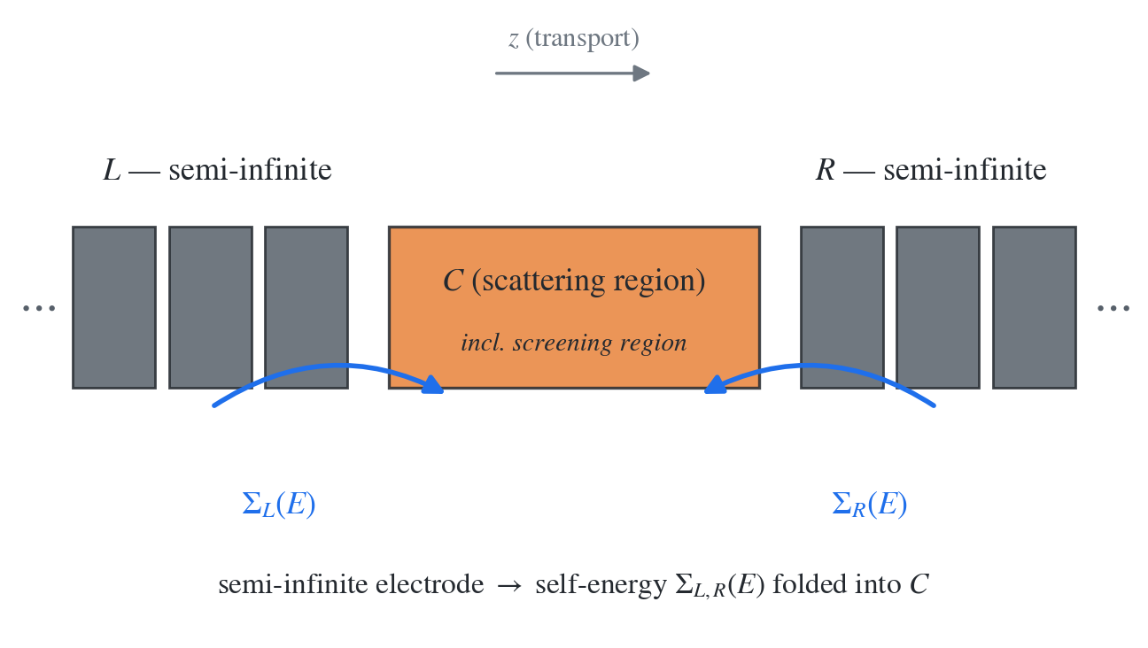
Figure 1. The L–C–R partition of an open system (schematic) — the semi-infinite electrodes are folded, via self-energies $\Sigma_{L,R}(E)$, into the finite central region $C$ (including the screening region), turning the infinite matrix problem into a finite one.

2. Why a local-orbital (LCAO) basis?

For the block partition above to hold, the basis functions must have finite range in real space. SIESTA's numerical atomic orbitals are exactly zero beyond a specified radius, so the Hamiltonian and overlap matrices are sparse, and "which atomic block interacts with which atomic block" is unambiguous. Therefore

1. the L–D–R spatial partition can be mapped directly onto a matrix block partition, and
2. the semi-infinite boundary condition of the electrodes can be handled through a recursion relation over periodic blocks (the surface Green's function).

In contrast, plane-wave basis functions are spread over the entire cell, so the very notion of spatial attribution — "this basis function belongs to the left electrode" — is impossible, and since periodic boundary conditions are presupposed, a semi-infinite electrode cannot be represented. This is why NEGF transport is handled by the SIESTA family (LCAO), while VASP (plane-wave) handles structure optimization and the reference electronic structure (Chapter 03). A workaround exists in which localized Wannier functions are constructed from plane-wave calculations and used in NEGF, but it is not covered in this tutorial.

3. The retarded Green's function

The retarded Green's function of the device region is defined as follows.

$$G(E) = \bigl[(E + i\eta)\,S - H - \Sigma_L(E) - \Sigma_R(E)\bigr]^{-1}$$

Here $H$ and $S$ are the Hamiltonian and overlap matrices of the device block ($S$ enters explicitly because the LCAO basis is non-orthogonal), $\Sigma_{L,R}$ are the electrode self-energies defined in the next section, and $\eta$ is a small positive number. Compared with the closed-system Green's function $[(E+i\eta)S - H]^{-1}$, which has poles at the eigenvalues of $H$, in the open system $\Sigma$ pushes those poles into the complex plane — the levels shift (real part of the self-energy) and acquire finite width (imaginary part). The size of $G(E)$ is the device matrix dimension (the number of orbitals), so the infinite open-system problem has been reduced to one inversion of a finite matrix per energy.

4. Self-energy — the infinite electrode as a finite matrix

Eliminating (downfolding) the left electrode block adds the following term to the device block.

$$\Sigma_L(E) = \tau_L(E)\, g_L(E)\, \tau_L^\dagger(E), \qquad \tau_L(E) = H_{DL} - E\,S_{DL}$$

$g_L(E)$ is the surface Green's function of the semi-infinite left electrode, computed recursively from the $H$ and $S$ of the electrode unit cell. Because the electrode is periodic, there is no need to actually invert an infinite matrix — the cell-by-cell recursion can be converged instead. This is why Chapter 05 performs a separate electrode calculation and stores its Hamiltonian (the TSHS file). $\Sigma_R$ works the same way.

The self-energy is in general an energy-dependent, non-Hermitian matrix, and its physics splits into two parts.

• Real part — the coupling to the electrode shifts the device levels (level shift).
• Imaginary part — it gives the levels a finite lifetime, because electrons do not stay in the device forever but can escape into the electrodes.

The imaginary part, taken separately, defines the broadening matrix.

$$\Gamma_\alpha(E) = i\bigl[\Sigma_\alpha(E) - \Sigma_\alpha^\dagger(E)\bigr], \qquad \alpha = L, R$$

$\Gamma_\alpha$ is a Hermitian matrix and is the matrix generalization of the coupling strengths $\gamma_{1,2}$ of the single-level model in Chapter 00. The relation between the level width $\gamma$ and the lifetime $\tau = \hbar/\gamma$ carries over unchanged.

5. The spectral function and the DOS

The anti-Hermitian part of the Green's function is the spectral function.

$$A(E) = i\bigl[G(E) - G^\dagger(E)\bigr] \;\xrightarrow{\ \eta \to 0\ }\; G\,(\Gamma_L + \Gamma_R)\,G^\dagger$$

The spectral function is the object containing "the states the device offers at energy $E$", and it splits naturally into electrode-resolved contributions.

$$A = A_L + A_R, \qquad A_\alpha = G\,\Gamma_\alpha\,G^\dagger$$

$A_L$ is the spectral density of the scattering states formed in the device by injection from the left electrode. The density of states (DOS) is obtained in a non-orthogonal basis by inserting the overlap.

$$\mathrm{DOS}(E) = \frac{1}{2\pi}\,\mathrm{Tr}\bigl[A(E)\,S\bigr]$$

The device DOS and spectral DOS (ADOS) output by TBtrans are exactly these quantities (Chapter 07).

6. Transmission — the Caroli formula

The transmission function is expressed in terms of the Green's function and the two broadening matrices.

$$T(E) = \mathrm{Tr}\bigl[\Gamma_L(E)\, G(E)\, \Gamma_R(E)\, G^\dagger(E)\bigr]$$

This expression is called the Caroli formula (Caroli et al. [2]). How to read it: it is the total amplitude for being injected from the left electrode ($\Gamma_L$), propagating through the device ($G$), and escaping into the right electrode ($\Gamma_R$). Inserting the resulting $T(E)$ into the Landauer integral

$$I = \frac{2e}{h}\int T(E)\,\bigl[f_L(E) - f_R(E)\bigr]\,dE$$

yields the current (Chapter 08). Diagonalizing $T(E)$ into channel-resolved contributions is the eigenchannel analysis (Chapter 10).

7. $\eta$ — a numerical parameter, not a physical quantity

In the $E + i\eta$ of the definition of $G(E)$, $\eta$ is an infinitesimal that selects the retarded solution (the causal branch), and in numerical calculations a finite value must inevitably be used. Let this be clear: $\eta$ is not a physical quantity. Physical broadening is carried by the imaginary part of the self-energy ($\Gamma$); $\eta$ is merely a numerical parameter that stabilizes the calculation.

• If $\eta$ is too large, every spectral structure is artificially smeared by a width $\eta$. 1D systems, with their many van Hove singularities and sharp resonances, are especially sensitive.
• If $\eta$ is small, the energy grid must be correspondingly fine. If the grid cannot resolve structures of width $\eta$, the spectrum looks jagged. The standard for this tutorial is $\eta = 0.001\ \mathrm{eV}$ (TBT.Contours.Eta of TBtrans), and the energy grid spacing is taken at or below $\eta$.

The $\eta$ convergence test is covered separately in Advanced: η broadening.

8. Division of labor between TranSIESTA and TBtrans

The formulas so far assumed the Hamiltonian $H$ was given. But in DFT, $H$ is a functional of the electron density, and the density of the open system in turn comes from the Green's function.

$$\rho = \frac{1}{2\pi}\int dE\,\bigl[A_L(E)\,f_L(E) + A_R(E)\,f_R(E)\bigr]$$

This equation is where the "NE (non-equilibrium)" of NEGF actually operates. Under bias, states injected from the left are filled up to $\mu_L$ and states injected from the right up to $\mu_R$ — a genuinely non-equilibrium density that cannot be described with a single Fermi level. Hence a self-consistent loop $\rho \to H[\rho] \to G \to \rho$ must be iterated, and this is the job of TranSIESTA. In practice the integral is split into an equilibrium part (computed stably on a complex contour) and a non-equilibrium part in the bias window (computed near the real axis, numerically delicate).

Once the converged $H$ is in hand, spectral quantities such as $T(E)$, DOS, and PDOS can be extracted without self-consistency, just by evaluating the Green's function at each energy. This is the job of TBtrans; it is far cheaper and can be rerun freely with different energy grids, $\eta$, and k-grids.

Code	What it does	Products
TranSIESTA	Self-consistent SCF with open boundary conditions + (at finite bias) the non-equilibrium density	Converged $H$ (TSHS), density (TSDE)
TBtrans	Post-processing transport on top of the converged $H$	$T(E)$, DOS, PDOS (TBT.nc)

At 0 V, $f_L = f_R$, so TranSIESTA is effectively an "open-boundary-condition SCF" (Chapter 06); only at finite bias does the non-equilibrium term switch on (Chapter 09).

Key summary

Object	Definition	Physical meaning
$G(E)$	$[(E+i\eta)S - H - \Sigma_L - \Sigma_R]^{-1}$	Retarded propagator of the open device
$\Sigma_\alpha(E)$	$\tau_\alpha\, g_\alpha\, \tau_\alpha^\dagger$	Effect of the semi-infinite electrode $\alpha$ (level shift + lifetime)
$\Gamma_\alpha(E)$	$i(\Sigma_\alpha - \Sigma_\alpha^\dagger)$	Broadening due to coupling to electrode $\alpha$
$A(E)$	$i(G - G^\dagger) = A_L + A_R$	Spectral density, $\mathrm{DOS} = \mathrm{Tr}[AS]/2\pi$
$T(E)$	$\mathrm{Tr}[\Gamma_L G \Gamma_R G^\dagger]$	Left → right transmission probability (Caroli)
$\eta$	Numerical parameter in $E + i\eta$	Not a physical quantity. Set jointly with the grid spacing

Exercises

1. Single-level toy model. Let the device be a single orbital ($H = \epsilon$, $S = 1$) and take the wide-band approximation $\Sigma_\alpha = -i\gamma_\alpha/2$ (energy-independent). Derive $G(E)$, $\Gamma_\alpha$, and $T(E) = \dfrac{\gamma_L \gamma_R}{(E-\epsilon)^2 + \bigl(\tfrac{\gamma_L + \gamma_R}{2}\bigr)^2}$. Verify that for symmetric coupling ($\gamma_L = \gamma_R$) the resonance peak gives $T(\epsilon) = 1$ — no matter how weak the coupling, transmission on resonance is perfect.

2. Spectral function identity. Starting from $G^{-1} - (G^\dagger)^{-1} = -(\Sigma_L - \Sigma_L^\dagger) - (\Sigma_R - \Sigma_R^\dagger) + 2i\eta S$, show that $A = G(\Gamma_L + \Gamma_R)G^\dagger$ holds as $\eta \to 0$.

3. Effect of $\eta$. Suppose the resonance width of Problem 1 is $\gamma_L + \gamma_R = 2\ \mathrm{meV}$. Discuss qualitatively how the height and width of the $T(E)$ peak are distorted when computed with $\eta = 50\ \mathrm{meV}$, and propose an appropriate $\eta$ and energy grid spacing.

---

Ref: Datta [1]; Caroli et al. [2]; Brandbyge et al. [3]; Papior et al. [4].