07. TBtrans — T(E) and DOS/PDOS

Learning objectives

• Understand that TBtrans is a post-processing tool that computes the transmission $T(E)$ and the DOS from a converged TranSIESTA result.
• Write a minimal TBtrans.fdf that excludes heavy output options.
• Know the relation between the numerical broadening $\eta$ and the energy-grid spacing delta, and set them together.
• Extract $T(E)$, DOS, and PDOS from trans.TBT.nc with sisl and plot them on a log axis.
• Physically interpret the integer plateaus of the pristine chain and the dip created by N substitution.

Background: TBtrans is post-processing, not SCF

Given the Hamiltonian converged by the TranSIESTA SCF of Chapter 06 (trans.TSHS), the transmission is a simple evaluation of the Caroli formula

$$T(E) = \mathrm{Tr}\!\left[\, \Gamma_L(E)\, G(E)\, \Gamma_R(E)\, G^{\dagger}(E) \,\right]$$

There is no self-consistency here — TBtrans is a post-processing tool that reads the fixed $H$ and computes $G(E)$, $T(E)$, and the DOS on an energy grid. The implementation and input format follow Papior et al. [4]. The energy range and grid spacing can therefore be changed and rerun without redoing the SCF.

The DOS comes in two flavors. The Green function DOS ($-\mathrm{Im}\,\mathrm{Tr}[G S]/\pi$, TBT.DOS.Gf) contains all states of the device, while the spectral-function DOS (TBT.DOS.A) contains only the states injected from — and therefore reachable from — a specific electrode. Their difference diagnoses localized states (bound states) not coupled to the electrodes.

Input file: minimal TBtrans.fdf

Add the following file to the 0bias/ directory. The structure and electrode definitions are reused via %include input.fdf (input.fdf in turn includes TS.fdf, so the TS.Elecs blocks are read along with it).

0bias/TBtrans.fdf

# ------------------------------------------------------------
# 07. TBtrans — T(E) / DOS / PDOS (0 V)
# Minimal option set — heavy output options deliberately excluded
# ------------------------------------------------------------
%include input.fdf

TBT.Voltage    0.00000 eV
TBT.nc.write   T

# ----- output selection -----
TBT.DOS.Gf     T     # Green function DOS
TBT.DOS.Elecs  T     # electrode bulk DOS
TBT.DOS.A      T     # spectral function DOS
TBT.DOS.A.All  T     # spectral DOS of all electrodes
TBT.T.All      T     # transmission between all electrode pairs
TBT.PDOS       T     # orbital-projected DOS

# ----- region where the Green function is solved -----
%block TBT.Atoms.Device
  atom [5 -- 16]
%endblock TBT.Atoms.Device

# ----- energy grid and broadening -----
TBT.Contours.Eta  0.001 eV

%block TBT.Contours
  line
%endblock TBT.Contours

%block TBT.Contour.line
  from -3.00 eV to 3.00 eV
   delta 0.001 eV
    method mid-rule
%endblock TBT.Contour.line

Keyword	Meaning
TBT.Voltage	The bias TBtrans assumes. 0 here, since this is a 0 V calculation. At finite bias it must equal TS.Voltage on the TranSIESTA side (Chapter 09)
TBT.nc.write	Forces writing trans.TBT.nc for sisl post-processing
TBT.DOS.*, TBT.T.All, TBT.PDOS	Select the physical quantities stored in trans.TBT.nc
TBT.Atoms.Device	Atom range where the Green function is actually solved. Specifying only the scattering region 5–16, excluding the electrode-copy regions (1–4, 17–20), gives smaller matrices and a lighter calculation
TBT.Contours.Eta	Numerical broadening $\eta$ of the device Green function (next section)
TBT.Contour.line	Real-axis energy grid — from $-3$ eV to $+3$ eV relative to $E_F$ in 1 meV steps

Pitfall 1 — do not add heavy output options

Options such as TBT.T.Bulk, TBT.T.Eig, and TBT.Current.Orb inflate the nc file to several GB and easily cause out-of-memory (OOM) failures. In particular, eigenchannel information can be obtained entirely by sisl post-processing from the Green function/spectral function in trans.TBT.nc, without the text output (TBT.T.Eig) (Chapter 10), so it is deliberately excluded from this minimal set.

Pitfall 2 — placement of TBT.kgrid_Monkhorst_Pack

If %block TBT.kgrid_Monkhorst_Pack is placed inside TBtrans.fdf, the k-points along the transport direction are automatically reduced to 1. To control the TBtrans k-grid directly, this block must go at the very end of input.fdf. In this example $x$ and $y$ are vacuum, so a k-grid of effectively a single $\Gamma$ point is sufficient and the block itself is unnecessary; but for systems with bulk electrodes periodic in the transverse directions, ignoring this placement rule breaks k convergence without any warning.

η and delta are set together

$\eta$ is the numerical broadening entering the imaginary part of the Green function $G = [(E + i\eta)S - H - \Sigma_L - \Sigma_R]^{-1}$. Every spectral feature is smeared into a Lorentzian of width $\sim\eta$, so an excessive $\eta$ artificially lowers sharp resonances and suppresses $T(E)$. Conversely, if the energy-grid spacing delta is larger than $\eta$, features of width $\eta$ slip between the grid points. Therefore set delta smaller than or comparable to $\eta$ (delta $\lesssim \eta$). This example uses $\eta = 1$ meV and delta $= 1$ meV. The effect of the choice of $\eta$ on the results is treated quantitatively in the Advanced chapter.

Running

Prerequisites: 0bias/ must contain the converged trans.TSHS from Chapter 06, and the electrode ../01_electrode/Electrode.TSHS is still required.

cd work/0bias
tbtrans TBtrans.fdf > tbtrans.stdout

Output analysis

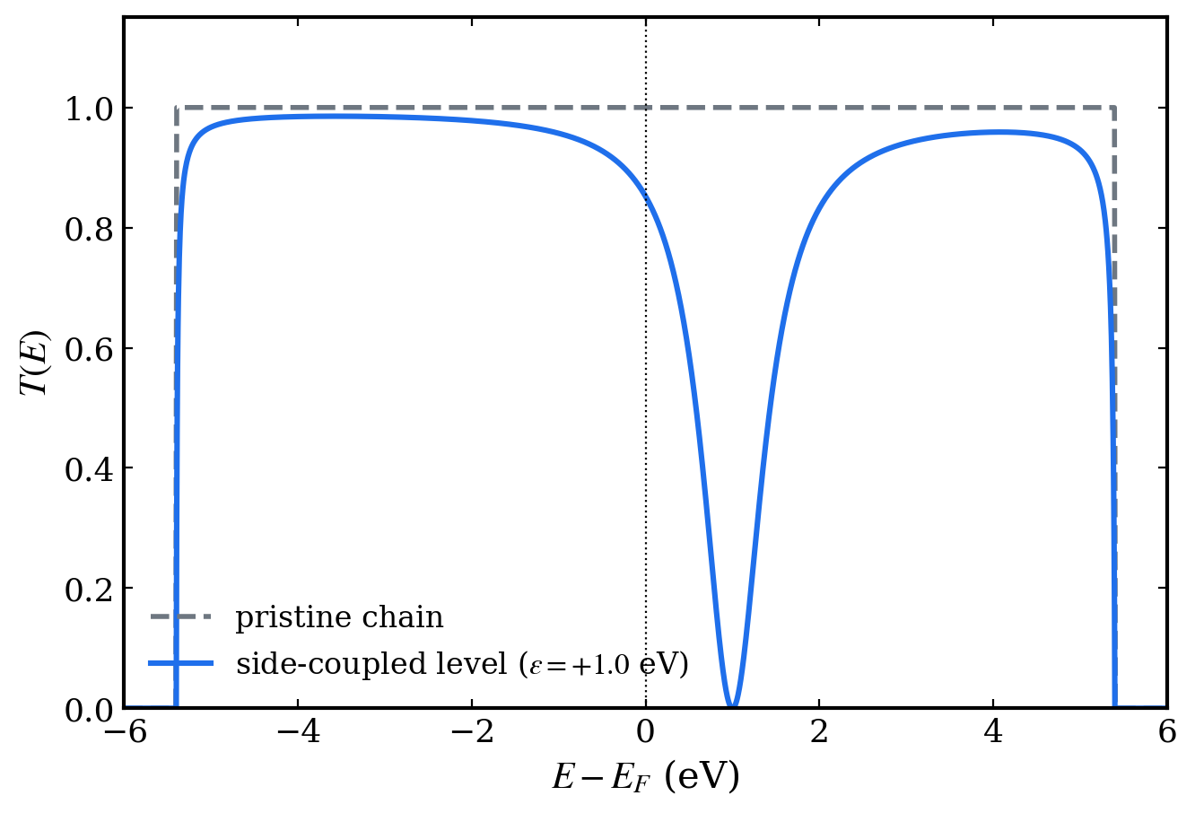
Figure 1. An actual NEGF calculation of a TB model — the $T=1$ plateau of a pristine chain (gray dashed) and the Fano antiresonance dip (blue) of a device where a localized level ($\epsilon=+1.0$ eV) couples to the chain. As a dip produced by an impurity level, this is the qualitative form of the result the C19N calculation of this chapter gives. (_scripts/fig_examples_batch.py)

tail -3 tbtrans.stdout
ls trans.TBT.nc

The single key output is trans.TBT.nc. This NetCDF container holds the energy grid, $T(E)$, the DOS, and the orbital-resolved DOS.

Extracting T(E), DOS, and PDOS with sisl

Parsing the text outputs (the AVTRANS family) is discouraged, because their energy-grid alignment and k-averaging are unclear. Reading trans.TBT.nc with sisl is the standard. sisl aligns energies as $E - E_F$ (eV) and applies k-averaging consistently.

plot_te.py

import numpy as np
import matplotlib.pyplot as plt
from sisl.io.tbtrans import tbtncSileTBtrans

t = tbtncSileTBtrans("trans.TBT.nc")

E = t.E                               # E - E_F (eV)
T = t.transmission(*t.elecs[:2])      # Left -> Right, k-averaged automatically

fig, ax = plt.subplots(figsize=(7, 6))
ax.semilogy(E, T)                     # T(E) spans several orders of magnitude, so a log axis is the default
ax.set_xlabel(r"$E - E_F$ (eV)")
ax.set_ylabel(r"$T(E)$")
fig.savefig("TE.png", dpi=300, bbox_inches="tight")

The DOS and PDOS come from the same file. The only caveat is that sisl atom indices are 0-based — atom 11 (N) in the fdf is 10 in sisl.

plot_dos.py

dos_gf = t.DOS()                # Green function DOS (entire device region)
ados_L = t.ADOS(t.elecs[0])     # spectral DOS injected from the Left electrode

# atom projections — the N atom only / the remaining C atoms only
dos_N = t.DOS(atoms=[10])
dos_C = t.DOS(atoms=[a for a in range(4, 16) if a != 10])

Energies where dos_gf differs strongly from the sum of ados (Left + Right) signal localized states not coupled to the electrodes.

Physical interpretation: plateaus and dips

There are two references for reading $T(E)$.

• Integer plateaus of the pristine chain. For a defect-free periodic chain, $T(E)$ equals the number of bands (channels) open along the transport direction at that energy — in the ballistic limit, transmission amounts to counting the open channels. An equally spaced carbon chain has a doubly degenerate $\pi$ band crossing near $E_F$, so a $T(E_F) = 2$ plateau is expected.
• The dip created by N substitution. The substituted atom acts as a scattering potential and causes backscattering in the $\pi$ channels. $T(E)$ drops below the plateau, and near the N-induced quasi-localized level a resonance–antiresonance structure (a sharp dip) appears. How much is carved out of the plateau is a direct measure of the scattering strength.

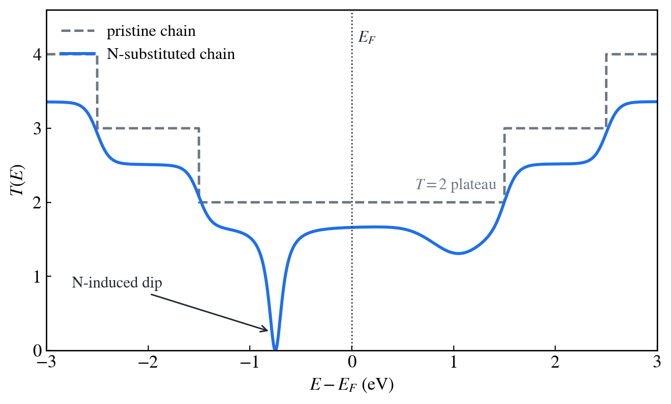
Figure 2. The two references for reading $T(E)$ (schematic, not a computed result) — the pristine chain shows integer plateaus counting the open channels ($T = 2$ near $E_F$), while the N-substituted device is suppressed below the plateau with a sharp antiresonance dip near the N level.

As an exercise, overlaying the $T(E)$ of a pristine device with N reverted to C on the same axes makes the difference between the two pictures clear.

Exercises

1. Increase delta from 0.001 eV to 0.01 eV, rerun, and compare how the depth and width of the N dip change. Explain the result through the relation between delta and $\eta$.
2. Repeat Chapters 06–07 with a pristine C20 device (N reverted to C) and overlay the two $T(E)$ curves to confirm the integer plateau and the dip.
3. Widen TBT.Atoms.Device to all atoms 1–20 and rerun. Observe whether $T(E)$ changes and how the computation time and memory change, and explain why.