05. The Electrode Calculation — Electrode.TSHS

Learning objectives

• Explain the role the electrode plays in an NEGF calculation — the periodic unit cell of the semi-infinite lead and the raw material of the self-energy.
• Judge, from orbital reach, the conditions the electrode unit cell must satisfy (no hopping beyond adjacent cells, atomic arrangement identical to the device boundary).
• Write an electrode input.fdf and run siesta to generate Electrode.TSHS.
• Set up the directory structure in which the generated Electrode.TSHS is shared, via path reference, by all subsequent device and bias calculations.

Background: the electrode is the raw material of the self-energy

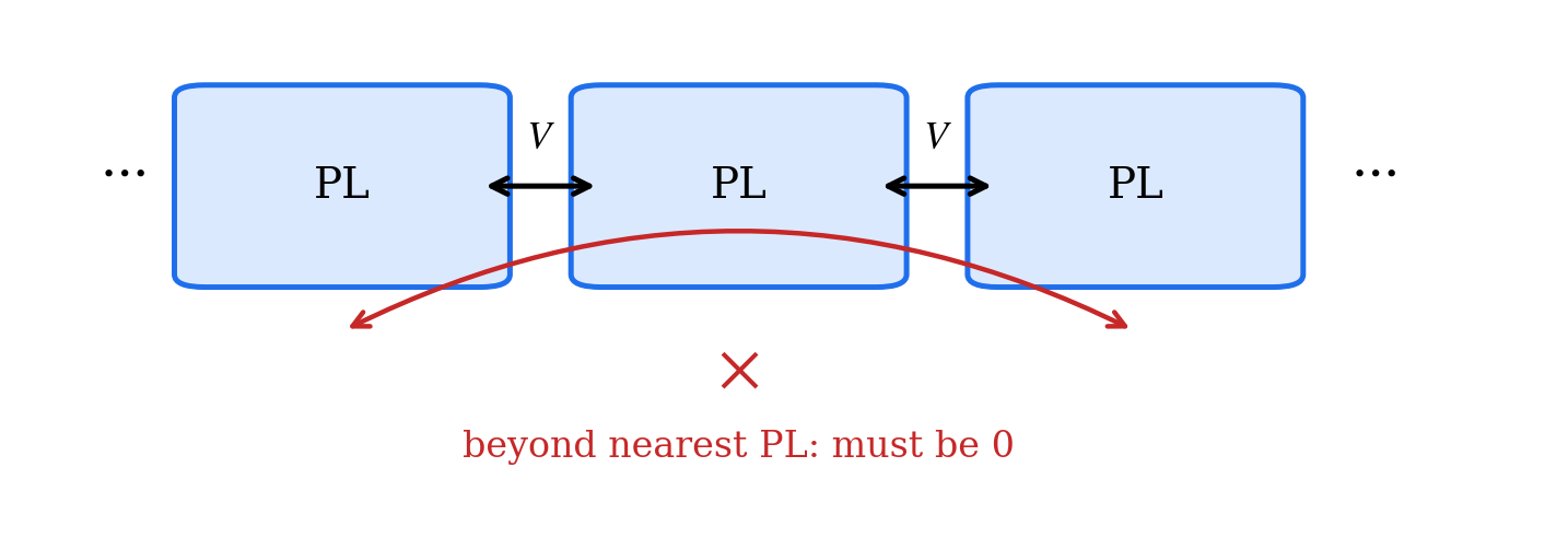
Figure 1. The principal layer condition — only the hopping $V$ between adjacent layers may remain, and coupling beyond that must be zero, for the semi-infinite electrode to be folded recursively. This is why the electrode cell is taken long enough along the transport direction. (Schematic)

Rewriting the device Green function derived in Chapter 04,

$$G(E) = \Big[ (E + i\eta)\,S - H - \Sigma_L(E) - \Sigma_R(E) \Big]^{-1}$$

Here $\Sigma_{L}(E)$ and $\Sigma_{R}(E)$ are the self-energies that fold the influence of the entire left and right semi-infinite electrodes on the finite scattering region into finite-size matrices. An infinitely long electrode cannot be handled directly, but if the electrode is a perfect crystal, the surface Green function can be constructed recursively from the Hamiltonian $H$ and overlap $S$ of a single periodic unit cell alone, and $\Sigma_{L/R}$ follows from it. The goal of this chapter is to produce exactly that raw material — the Electrode.TSHS file containing the $H$ and $S$ of the electrode unit cell.

The broadening matrices derived from the electrodes, $\Gamma_{L/R} = i\,(\Sigma_{L/R} - \Sigma_{L/R}^{\dagger})$, become the core ingredient of the transmission $T(E)$ calculation later (Chapter 07).

Figure 2. The cumulene electrode unit cell (4 C atoms, $d = 1.29$ Å, rendered from input.fdf) repeated 3 times along the transport direction — the electrode is a perfect periodic crystal in which this cell continues semi-infinitely.

Three conditions on the electrode unit cell

1. Perfect periodicity along the transport direction. The electrode must be an ideal crystal. Defects and substitutions belong only in the scattering region (Chapter 06).

2. No hopping beyond adjacent cells. The surface Green function recursion rests on the assumption that a unit cell couples only to its immediate neighbors (the principal layer). Because LCAO orbitals are exactly zero beyond a finite cutoff radius, this condition can be judged rigorously. The Hamiltonian/overlap element between two atoms is exactly zero if the interatomic distance exceeds the sum of the two orbital cutoff radii (roughly around 5 Å for DZP carbon). In the 4-atom C cell ($c = 5.16$ Å), the distance between the last atom of cell $n$ and the first atom of cell $n+2$ is $6.45$ Å, longer than this reach, so hopping beyond adjacent cells vanishes — a 4-atom cell is sufficient for the carbon chain electrode. In contrast, with a 2-atom cell ($c = 2.58$ Å) the same distance is $3.87$ Å, within the reach, so it cannot be used as an electrode. If the condition is borderline, lengthening the cell along the transport direction is the safe choice.

3. Atomic arrangement identical to the device boundary. Both ends of the device must have exactly the same atomic species, spacing, and lattice as the electrode unit cell so that they join smoothly onto the bulk electrode at the boundary. The device of Chapter 06 is built by replicating this electrode cell verbatim at both ends.

k-grid and parameter matching

The electrode is a periodic calculation with metallic bands along the transport direction ($z$), so the $z$-direction k-points must be dense (in this example $1\times1\times64$) to integrate the band filling and the Fermi level accurately. $x$ and $y$ are directions isolated by 15 Å of vacuum, so a single point suffices.

Furthermore, the electrode and the device must have identical values for the parameters that determine the Hamiltonian — basis (DZP), XC functional (PBE), MeshCutoff, electronic temperature, etc. If the electrode TSHS and the device Hamiltonian are produced under different conditions, the boundary junction is not physically valid.

Input file

The working tree starts as follows. The electrode is isolated in the 01_electrode/ directory.

work/
└── 01_electrode/
    ├── input.fdf
    └── C.psml        # PseudoDojo PBE pseudopotential

The structure is exactly the 1D carbon chain of Chapter 01 ($d = 1.29$ Å, $x=y=15$ Å vacuum), with the single line TS.HS.Save T added.

01_electrode/input.fdf

# ------------------------------------------------------------
# 05. Electrode — 1D carbon chain, 4-atom periodic cell
# Purpose: generate the H/S matrices (Electrode.TSHS) of the
#          electrode periodic along the transport direction (z)
# ------------------------------------------------------------
SystemName   C4 chain electrode
SystemLabel  Electrode

# ----- structure -----
NumberOfAtoms    4
NumberOfSpecies  1
%block ChemicalSpeciesLabel
  1  6  C
%endblock ChemicalSpeciesLabel

LatticeConstant 1.0 Ang
%block LatticeVectors
  15.000   0.000   0.000
   0.000  15.000   0.000
   0.000   0.000   5.160
%endblock LatticeVectors

AtomicCoordinatesFormat Ang
%block AtomicCoordinatesAndAtomicSpecies
  7.500  7.500  0.000  1
  7.500  7.500  1.290  1
  7.500  7.500  2.580  1
  7.500  7.500  3.870  1
%endblock AtomicCoordinatesAndAtomicSpecies

# ----- basis / XC / real-space grid -----
PAO.BasisSize    DZP
XC.Functional    GGA
XC.Authors       PBE
MeshCutoff       300. Ry

# ----- k-grid: dense only along the transport direction (z) -----
%block kgrid_Monkhorst_Pack
   1   0   0    0.0
   0   1   0    0.0
   0   0  64    0.0
%endblock kgrid_Monkhorst_Pack

# ----- SCF -----
MaxSCFIterations   300
SCF.DM.Tolerance   1.0d-8
SCF.Mixer.Weight   0.2
SCF.Mixer.History  15

# ----- TranSIESTA electrode output -----
TS.HS.Save  T

Keyword	Meaning
SystemLabel Electrode	Prefix of all products. The TSHS file name becomes Electrode.TSHS
LatticeVectors	$z = 5.16$ Å = 4 atoms $\times$ 1.29 Å. $x$, $y$ are 15 Å vacuum
PAO.BasisSize DZP and below	The parameter set that must be kept identical to the device
kgrid_Monkhorst_Pack	$1\times1\times64$ — dense sampling for the band integration along the transport direction
SCF.DM.Tolerance 1.0d-8	Density matrix convergence criterion. A loose value breaks the reliability of energy comparisons in later stages
TS.HS.Save T	Save the Hamiltonian/overlap as Electrode.TSHS after SCF convergence

Running

The electrode calculation is a plain siesta run. It is not TranSIESTA mode; the only difference is that a TSHS file is additionally saved due to TS.HS.Save T.

cd work/01_electrode
siesta < input.fdf > siesta.stdout

Analyzing the output

Verify normal termination and product generation.

tail -3 siesta.stdout      # normal-termination lines
ls Electrode.TSHS          # electrode H/S file

>> End of run:  ...
Job completed

Job completed at the end of stdout indicates normal termination. Besides Electrode.TSHS, the directory also contains Electrode.DM (density matrix), Electrode.XV (structure), and so on. Electrode.TSHS holds the converged $H$, $S$ along with the lattice and atomic information, and TranSIESTA and TBtrans construct the self-energy directly from this file.

Electrode.TSHS is referenced by path, not copied

All subsequent device and bias calculations reference this file via the relative path ../01_electrode/Electrode.TSHS rather than copying it into their own directories (the TS.Elec block of Chapter 06). Keeping the electrode in one place as the single authoritative copy guarantees the consistency that the entire bias chain (Chapter 09) uses the same electrode, and also makes it clear which calculations are affected when the electrode is changed.

Exercises

1. Suppose the electrode cell is reduced to 2 atoms ($c = 2.58$ Å). Compute the minimum distance between an atom of cell $n$ and an atom of cell $n+2$, compare it with the DZP orbital reach, and argue that electrode condition 2 is violated.
2. Find the cutoff radius of each C orbital in siesta.stdout and reconstruct, with actual numbers, the "interaction reach of about 5 Å" argument in the text.
3. Recompute the electrode with the k-grid reduced to $1\times1\times8$ and proceed through Chapter 07. Explain what artificial structures appear in $T(E)$ and what causes them.