08. I–V characteristics — Landauer integration and the symmetric bias window

Chapter 07 produced the transmission $T(E)$ of the C19N chain. This chapter feeds that $T(E)$ into the Landauer formula to compute the I–V curve. The calculation itself is a Python integration, but a single convention — where the bias window is placed — governs the physical interpretation of the result. Why the symmetric window is standard, and what artificial rectification signal an asymmetric window creates, are the core of this chapter.

Learning objectives

• Understand the meaning of the zero-bias approximation — integrating a fixed $T(E)$ over a bias window — and the limits of its applicability.
• Explain the rationale for the symmetric bias window $\mu_{L,R} = E_F \pm eV/2$.
• Identify the mechanism by which an asymmetric window produces an artificial rectification signal in a symmetric junction.
• Read $T(E)$ from trans.TBT.nc with sisl and obtain the I–V curve by trapezoidal integration.
• Know the form of the finite-temperature extension (Fermi–Dirac weighting).

Theory — the zero-bias approximation and the Landauer integral

In the zero-temperature Landauer formula the Fermi-function difference $f_L - f_R$ becomes a step: 1 between the two chemical potentials and 0 outside. The current is therefore the integral of $T(E)$ over the bias window.

$$I(V) = \frac{2e}{h}\int_{\mu_R}^{\mu_L} T(E)\,dE$$

Using as $T(E)$ the transmission of the Hamiltonian converged at 0 V is the zero-bias approximation. It is the low-voltage approximation of the Landauer picture [1] and assumes that $T(E)$ does not change when a bias is applied. It is therefore valid only for systems with small bias and good screening. To include the deformation of $T(E)$ with bias, a self-consistent calculation must be redone at every bias — that is the finite-bias TranSIESTA of Chapter 09.

The symmetric bias window

The two ends of the window are placed symmetrically.

$$\mu_L = E_F + \frac{eV}{2}, \qquad \mu_R = E_F - \frac{eV}{2}$$

This choice is equivalent to assuming that "when a bias is applied, the electrostatic potential drop is split evenly between the two sides of the junction, and the levels of the scattering region stay at the mean potential of the two electrodes." For a symmetric junction whose left and right are equivalent, this is the only self-consistent choice. An immediate consequence of the symmetric window is that, whatever the shape of the fixed $T(E)$,

$$I(-V) = \frac{2e}{h}\int_{+eV/2}^{-eV/2} T(E)\,dE = -I(V)$$

holds exactly. That is, under the zero-bias approximation with a symmetric window the I–V curve is always antisymmetric about the origin, and rectification cannot appear in principle.

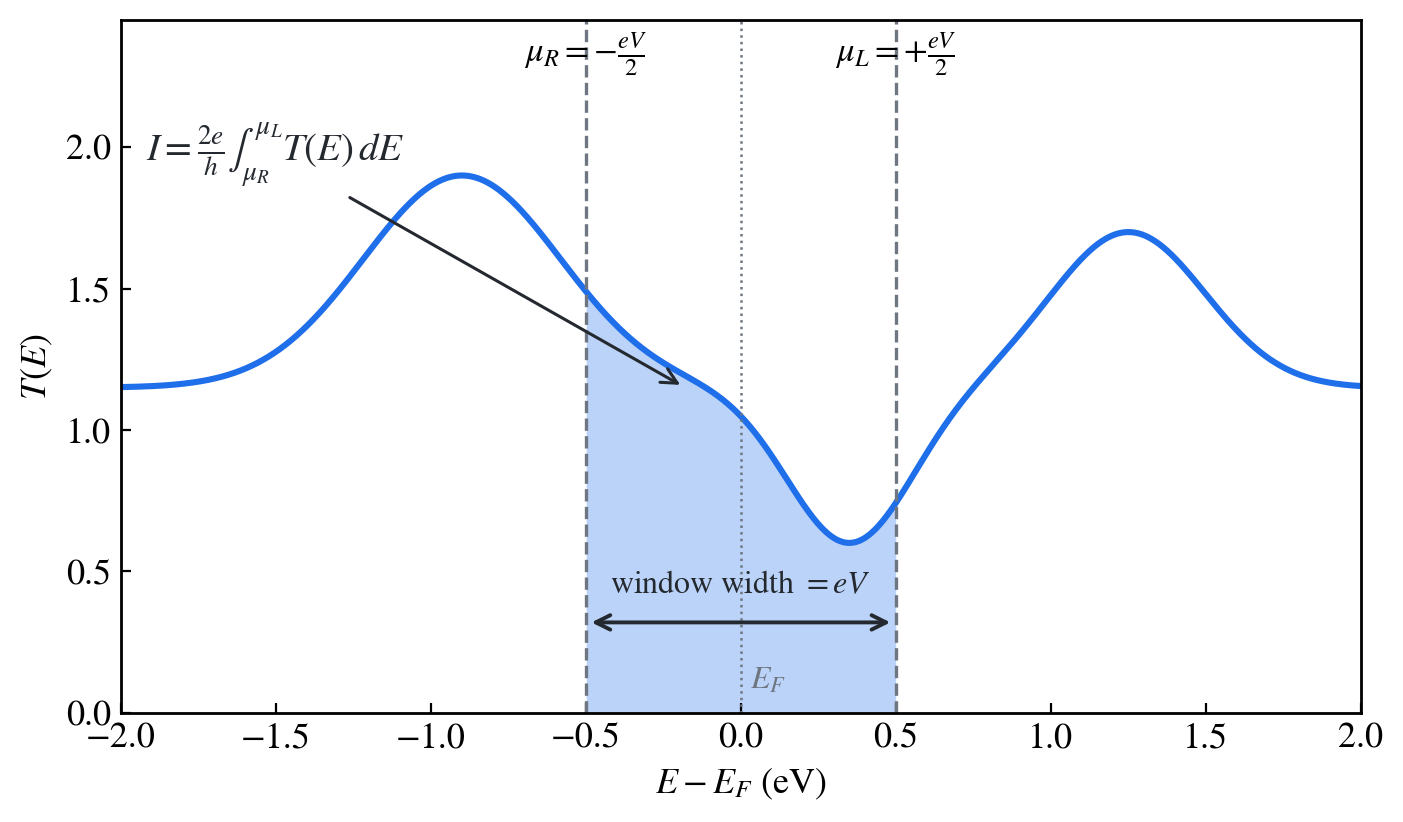
Figure 1. The symmetric bias window (schematic) — the current is the integral under the $T(E)$ curve over the interval $[\mu_R, \mu_L] = [E_F - eV/2,\ E_F + eV/2]$ (shaded), and the width of the integration window is $eV$.

Caution about the asymmetric window — an artificial rectification signal

Some legacy scripts use the asymmetric convention $\mu_L = E_F$, $\mu_R = E_F - eV$, which pins one electrode to ground. Performing the zero-bias-approximation integral with this convention gives

$$I(+V) \propto \int_{E_F - eV}^{E_F} T\,dE, \qquad I(-V) \propto -\int_{E_F}^{E_F + eV} T\,dE$$

so that positive bias integrates only the $T(E)$ below $E_F$ and negative bias only the $T(E)$ above $E_F$. If $T(E)$ is asymmetric about $E_F$ (as almost every real system is), then $|I(+V)| \neq |I(-V)|$, and this looks like a rectification ratio. But it is not physics — it is an artifact created by the integration convention. In the zero-bias approximation $T(E)$ is bias-invariant, so rectification in a symmetric junction is impossible in principle.

• If asymmetry appears in the I–V curve of a symmetric junction, suspect the window convention of the integration script before the result itself.
• Discussing rectification or NDC (negative differential conductance) requires a self-consistent finite-bias calculation (Chapter 09) in which $T(E)$ actually deforms with bias.

For reference, in a self-consistent finite-bias calculation $(0, -eV)$ and $(+eV/2, -eV/2)$ are gauge choices differing only in the overall potential reference, so the physics is the same. What matters is the window position in the zero-bias approximation, where a fixed $T(E)$ is integrated after the fact.

Finite temperature

At finite temperature the step is smoothed by the Fermi–Dirac distribution.

$$I(V) = \frac{2e}{h}\int T(E)\,\bigl[f(E-\mu_L) - f(E-\mu_R)\bigr]\,dE$$

The effect is a spreading of the window edges over a width $k_BT$ (about $25.9\ \mathrm{meV}$ at $300\ \mathrm{K}$). The difference between the two results is largest when a window edge crosses a sharp feature of $T(E)$ (a resonance or antiresonance).

Prerequisites

The 0bias/trans.TBT.nc produced by the TBtrans calculation of Chapter 07 is required. Following the tutorial standard, the energy grid is $[-3, 3]\ \mathrm{eV}$ with TBT.Contours.Eta 0.001 eV, and the grid spacing equals $\eta$ at 1 meV. The resolution of the window integral is tied directly to this grid, so if I–V is the goal it is best to make the grid sufficiently fine.

note

$T(E)$ is always read from trans.TBT.nc with sisl. The AVTRANS-family text output that TBtrans also writes requires separately verifying the energy alignment and k-averaging, so it is not parsed — the netCDF path handles the energy origin ($E - E_F$) and the k-averaging consistently.

Integration code

iv_zerobias.py

"""zero-bias approximation I-V: integrate T(E) from trans.TBT.nc over a symmetric bias window."""
import numpy as np
import sisl
from scipy.constants import e, h

tbt = sisl.get_sile("0bias/trans.TBT.nc")
E = np.asarray(tbt.E)                 # E - E_F (eV)
T = np.asarray(tbt.transmission())    # first two electrodes (Left -> Right)


def current_zero_bias(E, T, V, Ef=0.0):
    """Current (A) from integrating a fixed T(E) over the symmetric window [Ef - |V|/2, Ef + |V|/2].

    For a symmetric window the integration interval depends only on |V|, so the sign is applied last.
    I(-V) = -I(V) then holds automatically by convention.
    """
    if V == 0.0:
        return 0.0
    mu_L = Ef + 0.5 * abs(V)
    mu_R = Ef - 0.5 * abs(V)
    mask = (E >= mu_R) & (E <= mu_L)
    integral = np.trapz(T[mask], E[mask])   # integral in eV
    I = (2.0 * e / h) * integral * e        # trailing e: eV -> J conversion
    return np.sign(V) * I


bias = np.round(np.arange(-1.0, 1.001, 0.1), 3)
I = np.array([current_zero_bias(E, T, V) for V in bias])

np.savetxt("iv_zerobias.dat",
           np.column_stack([bias, I * 1e6]),
           header="V (V)    I (uA)")

import matplotlib.pyplot as plt
plt.plot(bias, I * 1e6, "o-")
plt.axhline(0.0, color="gray", lw=0.5)
plt.axvline(0.0, color="gray", lw=0.5)
plt.xlabel("V (V)")
plt.ylabel(r"I ($\mu$A)")
plt.savefig("iv_zerobias.png", dpi=200, bbox_inches="tight")

Line-by-line notes:

• tbt.E — the energy grid stored in the netCDF file. It is $E - E_F$ (eV) by TBtrans output convention, so Ef=0.0 is the Fermi level.
• tbt.transmission() — with arguments omitted, returns the k-averaged transmission between the first two electrodes (Left, Right).
• mask — selects only the grid points inside the window and integrates with np.trapz (trapezoidal rule). If a window edge falls between grid points the edge sliver is truncated, so the finer the grid the smaller the error (Exercise 3). From NumPy 2.0 on, use np.trapezoid instead of np.trapz.
• Units — in $\frac{2e}{h}\int T\,dE$ the integral was computed in eV, so multiplying once more by $e$ to convert to J gives the result in A. Multiply by 1e6 for $\mu$A and 1e9 for nA.

Running

cd 03_transport
python iv_zerobias.py
head iv_zerobias.dat

Output analysis

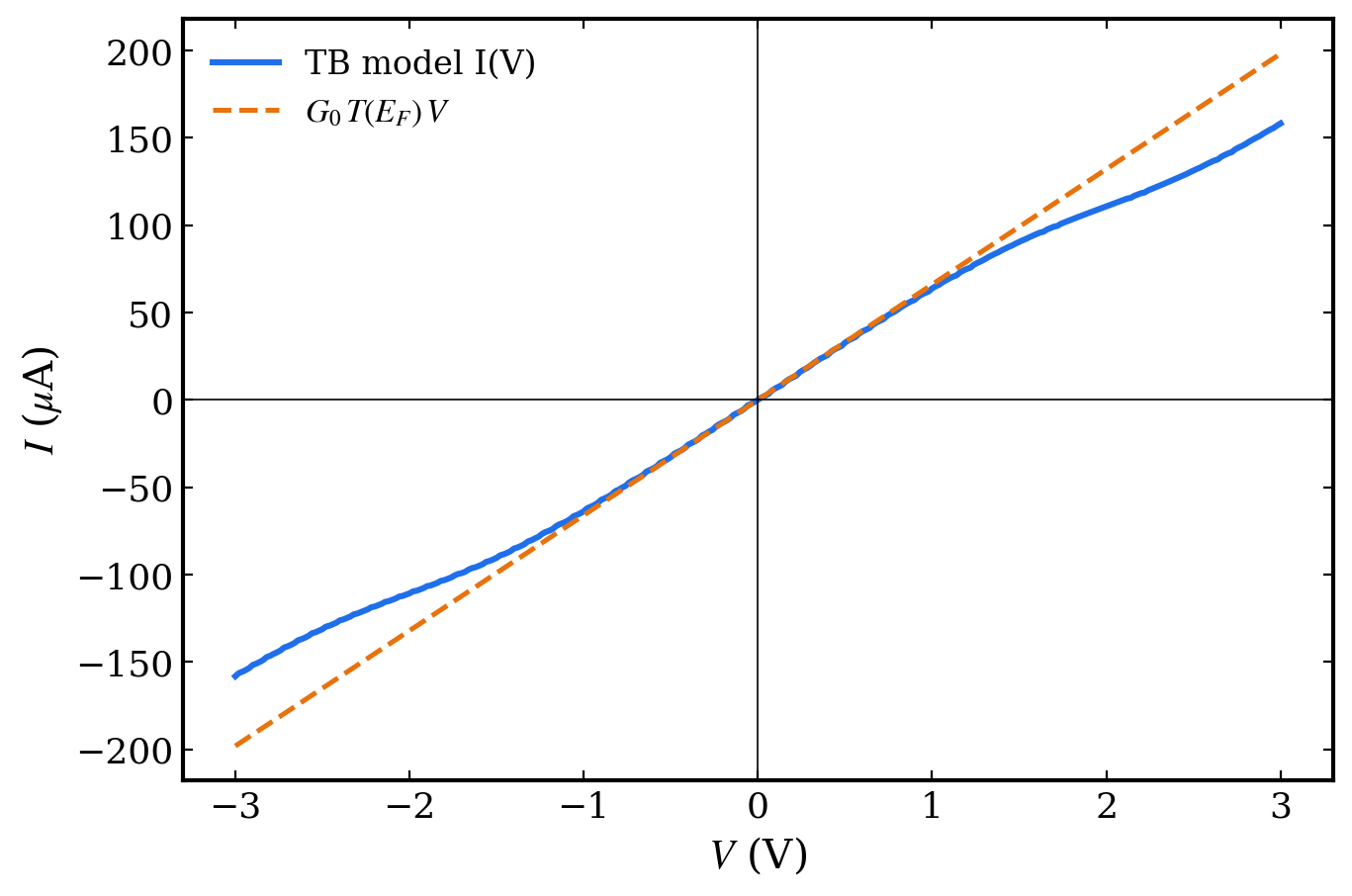
Figure 2. I–V obtained by integrating the TB-model $T(E)$ over a symmetric window — it is antisymmetric, $I(-V)=-I(V)$, and the low-bias slope matches the $G_0\,T(E_F)$ dashed line. (Actual TB-model calculation, _scripts/fig_examples_batch.py)

For the C19N chain (a symmetric junction with a single N atom at the center), the expected shape of the curve is as follows.

• Antisymmetry about the origin. $I(-V) = -I(V)$ must hold exactly within numerical error. If it is broken, check the window convention and the integration code first.
• Linear region at low bias. As $V \to 0$ the slope is $G = G_0\,T(E_F)$. For a pristine cumulene chain the two $\pi$ channels near $E_F$ give $T(E_F) = 2$ ($G = 2G_0$), but the N substitution scatters both channels so $T(E_F)$ is smaller than that. Check that the slope agrees with the $T(E_F)$ value obtained in Chapter 07. For a sense of magnitude: a channel with $T(E_F) = 1$ carries about $7.7\ \mu\mathrm{A}$ at $V = 0.1\ \mathrm{V}$.
• Slope changes. Whenever the window edges $\pm eV/2$ cross a peak or valley of $T(E)$ (the resonance structure created by the N impurity), the differential conductance $dI/dV$ changes. Mapping the kinks of the I–V curve by drawing the window on the $T(E)$ plot makes the structure of the zero-bias approximation clear.
• Limits of the zero-bias approximation. This curve has neither rectification nor NDC — it is a monotonic integral of a fixed $T(E)$. Whether it agrees with the finite-bias calculation (Chapter 09) at low bias, and how far the two diverge at high bias, tells you the validity range of the approximation.

Finite-T extension

Adding Fermi–Dirac weighting only smooths the window function; the structure is the same.

finite-T version

def current_finite_T(E, T, V, kT=0.02585, Ef=0.0):
    """Landauer current (A) including Fermi-Dirac weighting. Unit of kT: eV."""
    mu_L = Ef + 0.5 * V
    mu_R = Ef - 0.5 * V
    fL = 1.0 / (np.exp((E - mu_L) / kT) + 1.0)
    fR = 1.0 / (np.exp((E - mu_R) / kT) + 1.0)
    return (2.0 * e / h) * np.trapz(T * (fL - fR), E) * e

Since $f_L - f_R$ handles the sign automatically, no sign/abs treatment is needed, and the expression converges to the step window as $kT \to 0$. The only caveat is that the integration range must extend a few $k_BT$ beyond the window — the tutorial grid $[-3, 3]\ \mathrm{eV}$ is sufficient for a $\pm 1\ \mathrm{V}$ scan (window edges $\pm 0.5\ \mathrm{eV}$).

Exercises

1. Confirm the artificial rectification signal. Rewrite current_zero_bias for the asymmetric window ($\mu_L = E_F$, $\mu_R = E_F - eV$) and recompute the I–V curve from the same $T(E)$. Compute $|I(+1\,\mathrm{V})| / |I(-1\,\mathrm{V})|$ as a "rectification ratio", and explain which property of $T(E)$ it comes from and why it is not physical rectification.

2. Temperature effect. Overlay the $T = 0$ and $T = 300\ \mathrm{K}$ I–V curves on the same plot. At which bias is the difference between the two curves largest, and what feature of $T(E)$ is the window edge crossing at that point?

3. Grid convergence. Recompute the I–V curve from data thinned to every fifth point (E[::5], T[::5]) and plot the relative error against the original as a function of bias. Explain why the error is especially large at low bias in terms of the number of grid points inside the window.

---

Ref: S. Datta, Quantum Transport: Atom to Transistor (Cambridge UP, 2005); Chapter 07 (obtaining T(E)), Chapter 09 (self-consistent finite bias).