09. Finite bias — TS.Voltage and the bias chain

Learning objectives

• Explain the difference between the zero-bias approximation and a self-consistent finite-bias calculation, and judge when the latter is mandatory.
• Apply the file hand-off rules of a bias chain (stepping from 0 V up to the target voltage) — what must be copied and what must never be copied.
• Set both TS.Voltage and TBT.Voltage in each bias directory and verify them with grep.
• Understand the chemical-potential convention (symmetric $\pm V/2$) and how the contours reference the V symbol.
• Compare $T(E)$ across biases and read the current from the Currents block of the stdout.

Background: bias changes T(E) itself

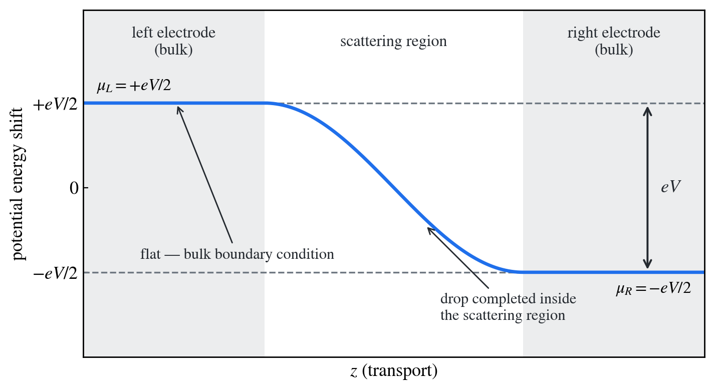
Figure 1. Potential profile at finite bias — both electrodes are pinned to bulk boundary conditions ($\pm eV/2$), and the voltage drop occurs inside the scattering region. This profile is exactly what TranSIESTA determines self-consistently. (Schematic)

The zero-bias approximation of Chapter 08 estimates the current by integrating the $T(E, V{=}0)$ computed at 0 V over the bias window.

$$I(V) \approx \frac{2e}{h} \int_{-V/2}^{+V/2} T(E, 0)\, dE$$

This approximation assumes the bias does not change the electronic structure. In reality, applying a voltage creates a potential drop in the scattering region, pushes the levels around, and deforms $T(E)$ itself into a function of $V$, $T(E, V)$. A self-consistent finite-bias calculation re-solves the NEGF SCF at each voltage and evaluates

$$I(V) = \frac{2e}{h} \int T(E, V)\, \big[ f(E - \mu_L) - f(E - \mu_R) \big]\, dE$$

The representative cases where the difference between the two results is essential are rectification and negative differential conductance (NDC). Rectification is the phenomenon in which an asymmetric structure makes the potential drop asymmetric so that $T(E, +V)$ and $T(E, -V)$ differ; NDC is the phenomenon in which the bias pushes resonant levels out of alignment so that the current decreases as the voltage increases. Neither can be reproduced in principle from $T(E, 0)$ alone.

At finite bias, TranSIESTA integrates the non-equilibrium density inside the bias window along a contour near the real axis (the TS.Contours.nEq of Chapter 06). That block, defined in advance at 0 V, is what is actually used here.

Bias chain: stepping up sequentially from 0 V

Applying the target voltage in one shot easily makes the SCF diverge. The standard procedure is a bias chain that inherits the converged state of the previous bias and raises the voltage stepwise. This example takes two steps: 0 V → 0.25 V → 0.5 V (the negative-bias chain branches separately from 0 V).

work/
├── 01_electrode/        # electrode master — shared by all biases via path reference
├── 0bias/               # completed state of Chapters 06–07
├── 0.25bias/            # starts by inheriting TSDE/DM/XV from 0bias
└── 0.5bias/             # starts by inheriting TSDE/DM/XV from 0.25bias

File hand-off rules

A new bias directory receives, along with the input files, only the converged-state files of the previous bias.

File	Handling	Reason
trans.TSDE	Must be copied	DM + energy DM. Without it the finite-bias calculation aborts with an error immediately at startup
trans.DM	Must be copied	SCF initial guess — accelerates convergence
trans.XV	Must be copied	Structure. Guarantees identical geometry between biases
*.ion, *.ion.nc, *.ion.xml	Optional	Basis-orbital cache — saves a little initialization time
trans.TSGFLeft, trans.TSGFRight	Must not be copied	Electrode self-energy cache — bias-dependent. Copying it crashes with a header mismatch
trans.TSCCEQ-*, trans.TSCCNEQ-*	Must not be copied	Contour checkpoints — per-bias cache
trans.KP, trans.TS.KP	Must not be copied	Per-bias k-point lists
H_MIXED*, trans.TSHS	Must not be copied	Regenerated automatically at the new bias
Electrode.TSHS	Not copied	Shared by path reference to ../01_electrode/ — Chapter 05

Starting a finite-bias run without the TSDE aborts immediately with the following error.

You have to calculate the 0 V and re-use the TSDE

The approach above — creating a fresh directory and copying only the required files — is the default. If instead an existing directory is cloned wholesale, the cache files on the must-not-copy list and the stale outputs of the previous calculation (stdout, MESSAGES, trans.STRUCT_OUT, etc.) must be deleted before starting.

Setting the voltage — edit two files together

There are two places to change in a new bias directory.

• TS.Voltage in TS.fdf → the target bias (for the TranSIESTA SCF)
• TBT.Voltage in TBtrans.fdf → the target bias (for TBtrans)

Pitfall — putting the voltage only in input.fdf leaves no bias applied

In fdf, when the same keyword is defined more than once only one definition takes effect. Even if you add TS.Voltage 0.25 eV to input.fdf, if the TS.Voltage 0.00000 eV left in TS.fdf remains effective the whole calculation runs at 0 V — and since the job terminates normally, it is hard to notice until you look at the results. Always edit the original definitions in TS.fdf and TBtrans.fdf directly, and verify with grep right after setting up.

grep -i voltage TS.fdf TBtrans.fdf input.fdf

Expected output — the bias value should appear only in TS.fdf and TBtrans.fdf, and not in input.fdf.

TS.fdf:TS.Voltage    0.25000 eV
TBtrans.fdf:TBT.Voltage    0.25000 eV

mu and the contours follow automatically

In the TS.fdf of Chapter 06 the chemical potentials were defined with the symmetric convention $\mu_{L} = +V/2$, $\mu_{R} = -V/2$ (the convention that pins one side at 0 and lowers the other to $-V$ is equivalent — only the potential reference differs), and the boundaries of the equilibrium and non-equilibrium contours are all written as TS.Voltage symbol references such as V/2 and |V|/2. Therefore changing the single TS.Voltage line automatically adjusts $\mu_{L,R}$ and every integration path to the new bias. The design structurally prevents the mistake of rewriting the mu values or contour boundaries as numbers for each bias.

Running

The full procedure for the 0.25 V step.

cd work
mkdir 0.25bias

# inputs + pseudopotentials
cp 0bias/input.fdf 0bias/TS.fdf 0bias/TBtrans.fdf 0.25bias/
cp 0bias/C.psml 0bias/N.psml 0.25bias/

# converged state of the previous bias (only the 3 must-copy files)
cp 0bias/trans.TSDE 0bias/trans.DM 0bias/trans.XV 0.25bias/

cd 0.25bias
# TS.fdf:      edit to TS.Voltage  0.25000 eV
# TBtrans.fdf: edit to TBT.Voltage 0.25000 eV
grep -i voltage TS.fdf TBtrans.fdf input.fdf   # proceed after verification

siesta < input.fdf > siesta.stdout
tbtrans TBtrans.fdf > tbtrans.stdout

For 0.5 V, repeat the same procedure but take TSDE/DM/XV from 0.25bias — the starting point is always the immediately preceding bias. Voltage steps of a few hundred mV or less, like the 0.25 V of this example, are safe; if the SCF struggles to converge, subdivide the steps further.

Output analysis

Current — the Currents block in the stdout

When the bias window is open, the Currents block near the end of the tbtrans stdout prints the current for each electrode pair.

grep -A3 -i "currents" tbtrans.stdout

# (schematic example — the exact format and numbers depend on version and system)
Currents:
  Left -> Right:  V = 0.25 V ;  I = 1.2E-05 A

As a cross-check, you can integrate $T(E, V)$ directly from the trans.TBT.nc of the same bias. In the low-temperature limit the current is the integral of $T(E)$ over the bias window $[\mu_R, \mu_L]$.

current_check.py

import numpy as np
from scipy.constants import e, h
from sisl.io.tbtrans import tbtncSileTBtrans

def current(path, V):
    t = tbtncSileTBtrans(path)
    E = np.asarray(t.E)                          # E - E_F (eV)
    T = np.asarray(t.transmission(*t.elecs[:2]))
    mu_L, mu_R = +0.5 * V, -0.5 * V
    mask = (E >= mu_R) & (E <= mu_L)
    integral = np.trapz(T[mask], E[mask])        # in eV
    return (2 * e / h) * integral * e            # A

print(current("0.25bias/trans.TBT.nc", 0.25))

The stdout value includes finite-temperature Fermi-function weighting, so it may differ slightly from the low-temperature integral.

Comparing T(E) across biases

The key output of a bias chain is the deformation of $T(E, V)$ itself. Overlay the $T(E)$ of the three biases.

plot_te_bias.py

import matplotlib.pyplot as plt
from sisl.io.tbtrans import tbtncSileTBtrans

cases = {"0 V":    "0bias/trans.TBT.nc",
         "0.25 V": "0.25bias/trans.TBT.nc",
         "0.5 V":  "0.5bias/trans.TBT.nc"}

fig, ax = plt.subplots(figsize=(7, 6))
for label, path in cases.items():
    t = tbtncSileTBtrans(path)
    ax.semilogy(t.E, t.transmission(*t.elecs[:2]), label=label)

ax.axvspan(-0.25, 0.25, alpha=0.1)    # 0.5 V bias window
ax.set_xlabel(r"$E - E_F$ (eV)")
ax.set_ylabel(r"$T(E)$")
ax.legend()
fig.savefig("TE_bias_compare.png", dpi=300, bbox_inches="tight")

There are two things to look for. First, how far $T(E, V)$ deviates from the 0 V curve inside the bias window — a small deviation is an a posteriori verification that the zero-bias approximation (Chapter 08) is justified for this system and this voltage range. Second, whether resonance features such as the N dip shift and deform with bias — this is the microscopic origin of NDC and rectification.

Exercises

1. Try starting 0.5 V directly in a new directory without trans.TSDE, and confirm the error message from the text in the stdout. Then copy the TSDE, rerun, and record the difference.
2. Skip 0.25 V and compute 0.5 V directly from the 0 V TSDE. Compare with the chain that went through 0.25 V: how does the number of SCF iterations change, and do the final results agree?
3. With the asymmetric device of Exercise 1 in Chapter 06 (N placed at atom 8), compute $\pm 0.5$ V and obtain the rectification ratio $\left| I(+V)/I(-V) \right|$. Interpret the result in terms of the difference between $T(E, +V)$ and $T(E, -V)$.