06. Device 0 V — TranSIESTA self-consistent NEGF

Learning objectives

• Explain how a device cell is composed of electrode-copy regions and a scattering region.
• Write device inputs split into input.fdf (structure, basis, SCF) and TS.fdf (TranSIESTA blocks).
• Read the roles and cross-reference structure of TS.ChemPots, TS.Elecs, and the contour blocks.
• Run the 0 V TranSIESTA SCF and verify convergence and the generation of trans.TSDE and trans.TSHS.
• Know which files the 0 V calculation must save to serve as the starting point of a finite-bias chain.

Background: the device is a scattering region sandwiched between electrodes

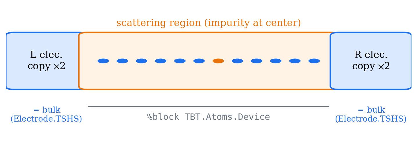
Figure 1. Device layout — the blocks at both ends are copies of the electrode unit cell, and the region between them is the scattering region. The electrode Hamiltonian is shared by a path reference to Electrode.TSHS, and the region where the Green function is solved is specified with TBT.Atoms.Device. (Schematic)

In a NEGF calculation the device (the scattering-region cell) consists of three parts.

 [ Left electrode copy ]  [ scattering region ]              [ Right electrode copy ]
   atoms 1–4 (C)            atoms 5–16 (C ... N ... C)         atoms 17–20 (C)
   z = 0.00–3.87             z = 5.16–19.35                     z = 20.64–24.51

• Electrode-copy regions: both ends of the device cell must be identical in atomic species, spacing, and arrangement to the electrode unit cell of Chapter 05. TranSIESTA stitches the Hamiltonian of this region to that of the electrode TSHS, so any deviation from the bulk electrode here produces artificial scattering at the boundary.
• Scattering region: where the object of interest — a defect, a molecule, an interface — resides. This example uses C19N, a 20-atom carbon chain whose central atom (atom 11, $z = 12.90$ Å) is substituted by N ($c = 25.8$ Å).
• The scattering-region atoms adjacent to the electrode boundaries must have enough margin (screening length) for the potential to recover its bulk value. A convergence test with respect to the scattering-region length is covered in the Advanced chapter.

Figure 2. C19N device structure (rendered from input.fdf, 20 atoms) — only the central atom 11 is N (blue); the rest are C (gray). The four atoms at each end form electrode-copy regions with the same arrangement as the electrode cell.

At 0 V the chemical potentials of the two electrodes are equal ($\mu_L = \mu_R = E_F$), but the calculation itself is already an open-boundary NEGF calculation. The self-consistent NEGF formalism of TranSIESTA follows Brandbyge et al. [3] and Papior et al. [4]. The density is obtained from a complex-plane contour integral of the Green function

$$\rho = -\frac{1}{\pi} \int \mathrm{Im}\, G(E)\, f(E)\, dE$$

and this is iterated through the SCF cycle. The 0 V result is itself the input to the transmission calculation (Chapter 07) and the starting point of the finite-bias chain (Chapter 09).

Input files

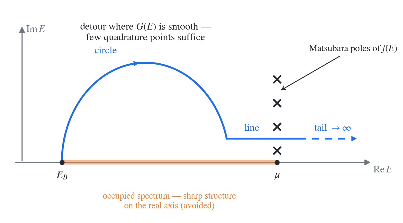
Figure 3. Complex-plane contour of the TranSIESTA equilibrium-density integral — instead of the real axis, the integration detours through the complex plane (circle + line + tail, $\times$ = poles), where the Green function is smooth. The TS.Contour blocks define this path. (Schematic)

The directory convention names bias directories alongside the electrode. The 0 V device is 0bias/.

work/
├── 01_electrode/
│   └── Electrode.TSHS      # output of Chapter 05 (shared by path reference)
└── 0bias/
    ├── input.fdf           # structure, basis, SCF + %include TS.fdf
    ├── TS.fdf              # TranSIESTA blocks
    ├── C.psml
    └── N.psml

Separation of roles: input.fdf holds what is common to any calculation (structure, basis, SCF settings), while TS.fdf holds the TranSIESTA-specific settings (voltage, chemical potentials, contours, electrode definitions). When changing the bias, only TS.fdf needs to be touched.

input.fdf

0bias/input.fdf

# ------------------------------------------------------------
# 06. Device — C19N chain, 20 atoms (atom 11 substituted by N), 0 V
# left 4 atoms + scattering region 12 atoms + right 4 atoms
#   = same arrangement as the electrode C4 cell
# ------------------------------------------------------------
SystemName   C19N chain device
SystemLabel  trans

NumberOfAtoms    20
NumberOfSpecies   2
%block ChemicalSpeciesLabel
  1  6  C
  2  7  N
%endblock ChemicalSpeciesLabel

LatticeConstant 1.0 Ang
%block LatticeVectors
  15.000   0.000   0.000
   0.000  15.000   0.000
   0.000   0.000  25.800
%endblock LatticeVectors

AtomicCoordinatesFormat Ang
%block AtomicCoordinatesAndAtomicSpecies
  7.500  7.500   0.000  1    #  1 - Left electrode copy
  7.500  7.500   1.290  1    #  2
  7.500  7.500   2.580  1    #  3
  7.500  7.500   3.870  1    #  4
  7.500  7.500   5.160  1    #  5 - scattering region
  7.500  7.500   6.450  1    #  6
  7.500  7.500   7.740  1    #  7
  7.500  7.500   9.030  1    #  8
  7.500  7.500  10.320  1    #  9
  7.500  7.500  11.610  1    # 10
  7.500  7.500  12.900  2    # 11 - N (cell center)
  7.500  7.500  14.190  1    # 12
  7.500  7.500  15.480  1    # 13
  7.500  7.500  16.770  1    # 14
  7.500  7.500  18.060  1    # 15
  7.500  7.500  19.350  1    # 16
  7.500  7.500  20.640  1    # 17 - Right electrode copy
  7.500  7.500  21.930  1    # 18
  7.500  7.500  23.220  1    # 19
  7.500  7.500  24.510  1    # 20
%endblock AtomicCoordinatesAndAtomicSpecies

# ----- basis / XC / grid — must be identical to the electrode -----
PAO.BasisSize    DZP
XC.Functional    GGA
XC.Authors       PBE
MeshCutoff       300. Ry

# transport-direction k is 1 — the open boundary is handled by the electrode self-energy
%block kgrid_Monkhorst_Pack
  1  0  0   0.0
  0  1  0   0.0
  0  0  1   0.0
%endblock kgrid_Monkhorst_Pack

MaxSCFIterations   500
SCF.DM.Tolerance   1.0d-8
SCF.Mixer.Weight   0.2
SCF.Mixer.History  15
SpinPolarized      T

# ----- what the finite-bias chain starting point must save -----
DM.UseSaveDM  T      # reuse the existing DM on restart
TS.HS.Save    T      # save trans.TSHS (TBtrans input)
Write.DM      T      # save trans.DM

%include TS.fdf

The 0 V calculation is the starting point of the finite-bias chain

Subsequent finite-bias calculations (Chapter 09) start by inheriting the 0 V trans.TSDE (density matrix + energy density matrix). The 0 V input.fdf must therefore contain DM.UseSaveDM T, TS.HS.Save T, and Write.DM T. Without these flags the TSDE/TSHS files are not written and the bias chain cannot be started.

TS.fdf

0bias/TS.fdf

# ------------------------------------------------------------
# TranSIESTA settings — 0 V (starting point of the finite-bias chain)
# Changing the single TS.Voltage line updates mu and all contours
# (they reference the V symbol)
# ------------------------------------------------------------
SolutionMethod  transiesta

TS.Voltage    0.00000 eV

# ----- chemical potentials: symmetric ±V/2 convention -----
%block TS.ChemPots
  Left
  Right
%endblock TS.ChemPots

%block TS.ChemPot.Left
  mu V/2
  contour.eq
    begin
      C-Left
      T-Left
    end
%endblock TS.ChemPot.Left

%block TS.ChemPot.Right
  mu -V/2
  contour.eq
    begin
      C-Right
      T-Right
    end
%endblock TS.ChemPot.Right

# ----- equilibrium contours (complex-plane integration path) -----
TS.Contours.Eq.Pole    2.50000 eV

%block TS.Contour.C-Left
  part circle
   from -40.00000 eV + V/2 to -10 kT + V/2
    points 25
     method g-legendre
%endblock TS.Contour.C-Left

%block TS.Contour.T-Left
  part tail
   from prev to inf
    points 10
     method g-fermi
%endblock TS.Contour.T-Left

%block TS.Contour.C-Right
  part circle
   from -40.00000 eV - V/2 to -10 kT - V/2
    points 25
     method g-legendre
%endblock TS.Contour.C-Right

%block TS.Contour.T-Right
  part tail
   from prev to inf
    points 10
     method g-fermi
%endblock TS.Contour.T-Right

# ----- non-equilibrium contour (actually used only at finite bias) -----
%block TS.Contours.nEq
  neq
%endblock TS.Contours.nEq

%block TS.Contour.nEq.neq
  part line
   from -|V|/2 - 5 kT to |V|/2 + 5 kT
    delta 0.01000 eV
     method mid-rule
%endblock TS.Contour.nEq.neq

# ----- electrode definitions -----
%block TS.Elecs
  Left
  Right
%endblock TS.Elecs

%block TS.Elec.Left
  HS ../01_electrode/Electrode.TSHS
  chemical-potential Left
  semi-inf-direction -a3
  electrode-position 1
%endblock TS.Elec.Left

%block TS.Elec.Right
  HS ../01_electrode/Electrode.TSHS
  chemical-potential Right
  semi-inf-direction +a3
  electrode-position end -1
%endblock TS.Elec.Right

Block-by-block notes:

Block/keyword	Meaning
SolutionMethod transiesta	Switches the siesta run to perform the NEGF SCF instead of diagonalization
TS.Voltage	Voltage between the electrodes. The mu values and contour boundaries below all reference this value through the symbol V, so this single line is the reference when changing the bias
TS.ChemPots + TS.ChemPot.Left/Right	Chemical-potential definitions. The symmetric convention $\mu_{L,R} = \pm V/2$ is used (pinning one side at 0 is also possible — Chapter 09). The list of equilibrium contours attached to each $\mu$ is given by contour.eq
TS.Contour.C-* / T-*	Equilibrium-density integration path — a circle in the complex plane and a Fermi tail. The boundaries are written with the V/2 symbol, so they follow the bias automatically
TS.Contours.nEq	Non-equilibrium density integration inside the bias window (near the real axis). At 0 V there is no window so it is effectively unused, but it is defined in advance so Chapter 09 can reuse it as is
TS.Elecs + TS.Elec.Left/Right	Electrode definitions. HS is a relative-path reference (not a copy) to the Chapter 05 output; chemical-potential links to the ChemPot name above; semi-inf-direction ±a3 is the semi-infinite direction; electrode-position locates the electrode-copy region (1 = starting from atom 1, end -1 = ending at the last atom)

Spin treatment

This C19N model has 81 valence electrons in total — an odd-electron system. The example therefore starts with SpinPolarized T, and the final magnetic moment and the spin-resolved transmission must be checked. If a non-magnetic solution is the goal, simplify to a non-spin calculation only after confirming that the final moment of the spin-polarized calculation is zero.

Running

First check that ../01_electrode/Electrode.TSHS exists. In SIESTA 5.x, TranSIESTA is not a separate executable but is integrated into siesta; running siesta with an input that sets SolutionMethod transiesta performs the TranSIESTA SCF.

cd work/0bias
ls ../01_electrode/Electrode.TSHS    # check the electrode is ready
siesta < input.fdf > siesta.stdout

If no prior density matrix exists, TranSIESTA generally first builds an initial density with an ordinary periodic-boundary SCF and then switches to the NEGF cycle. Both stages appear in order in the stdout.

Output analysis

Checking convergence

The TranSIESTA SCF log prints the density-matrix change (dDmax) and the Hamiltonian change (dHmax) at each iteration. The convergence criterion is SCF.DM.Tolerance ($10^{-8}$ in this example).

grep -c "ts-scf" siesta.stdout     # did the NEGF SCF cycle run?
tail -5 siesta.stdout              # normal-termination lines

>> End of run:  ...
Job completed

The Job completed on the last line is the criterion for normal termination. A calculation that stopped midway lacks this line. If dDmax oscillates rather than decreasing monotonically with iteration, lowering SCF.Mixer.Weight is the first remedy.

Checking the outputs

ls trans.TSHS trans.TSDE trans.DM trans.XV

File	Contents	Use
trans.TSHS	Converged device Hamiltonian/overlap	Input to TBtrans (Chapter 07)
trans.TSDE	density matrix + energy density matrix	Mandatory hand-off file for the finite-bias chain (Chapter 09)
trans.DM	density matrix	SCF initial guess for restarts and for the next bias
trans.XV	Final structure	Verifying identical geometry between biases

All four files must be present to proceed to the following chapters.

Exercises

1. Build an asymmetric device with N moved from atom 11 to atom 8 and repeat the 0 V calculation. This result is reused in the rectification discussion of Chapter 09.
2. Build a C27N device with an extended scattering region (28 atoms, $c = 36.12$ Å, N kept at the center), run the same calculation, and compare the number of SCF iterations required for convergence and the results. Scattering-region length convergence is the topic of the Advanced chapter.
3. In the TS.ChemPot blocks, change the $\mu$ convention from $\pm V/2$ to Left = 0 and Right = $-V$; check whether the 0 V result changes, and explain whether (or not) the difference between the two conventions affects physical quantities at finite bias.